
1 The Complexity of Algorithms Usually there are many programs or algorithms which can compute the solution of a specified task or problem.It is necessary,therefore,to consider those criteria which can be used to decide the best choice of program in various cir- cumstances.These criteria might include such properties of programs as good documentation,evolvability,portability and so on.Some of these can be analysed quantitatively and rigorously,but in general many of them cannot be evaluated precisely.Perhaps the most important criteria (after 'correctness',which we will take for granted)is what is loosely known as 'program efficiency'.Roughly speaking,the efficiency of a program is a measure of the resources of time and space (memory or store)which are required for its execution.It is desirable,of course,to minimise these quantities as far as possible,but before we can con- sider this it is necessary to develop a rigorous notation which can be used as a yardstick for our programs.It is the purpose of this chapter to introduce such a notation,along with some illustrative examples. 1.1 Comparing the Efficiency of Algorithms Let us consider a few examples that illustrate the differences in time and space requirements of different programs for a particular problem.Consider the follow- ing search problem: The array A[1..128]contains 128 integers in increasing order of magnitude (with no duplicates).Write a program to find the index i such that A[i]=C where C is a given integer constant.If there is no such i,a zero should be returned. A simple solution may start scanning the array from left to right (in ascend- ing order of index)until either a location is found which contains C or the end of the array is reached (see function search on page 3). Intuitively,it can be seen that,in the worst case,this sequential search may have to inspect each element of A.Now we can use the fact that the array is ordered to develop a new algorithm.We compare C with the middle element of the array A[64](in this case).If C=A[64],the solution is found.If C<A[64] then,if present,C must be in A[1]...A[63]and if C>A[64],it must be in A[65]...A[128].In either case,a search within a smaller sub-array should be initiated.Thus the function b_search can be developed: 2
The Complexity of Algorithms 3 const N 128; function search (C integer):integer; var J integer; begin J t=1;(x initialise J x) (x while end of list is not reached and c is not found,continue the search x) while (A[J]C)and (J<N)do J:=J+1; ifA[JJ】=c then search =J (关.,c is found and A【J】=C) e1 se search:=0(¥,.,c not found) end;(of search美) function bsearch (c integer):integer; var U,I,L integer; (x U and L are lower and upper indices x) (x of the array to be searched x) found boolean; begin L=1;U4=N; (x initialise the bounds of the array x) found :false; The array A[L]..A[U]is searched.While c is not found and the array is not empty the search continues x) while (not found)and (U >L)do begin I :(U L)div 2;(x find the middle of the array x) if C A[I]then found :true else if C>A[I】then L:=I+1 e1se(C<A[I】关) U1=I-1 end; if found then b_search =I else b_search :0 end;(x of bsearch x) This new algorithm is known as 'binary search',since it repeatedly divides the array into two equal-sized sub-arrays,until either C is found or the sub-array is empty.Informally,it can be seen that each time the body of the while loop is executed,the size of the array is reduced by half.So,the body of the loop is exe- cuted a maximum of seven times.That is,at most seven elements of the array have to be examined.This,of course,is an immense improvement over the sequential search which may have to look up 128 elements.These two functions, although they perform the same task,are radically different in the time they need to obtain the solution
4 Abstract Data Types and Algorithms Let us look at a second example.We wish to generate a sequence of numbers an(for a given n,n≥O): 01123581321.. where a0=0 41=1 an an-1+an-2 for n>1. Again,we can develop different solutions to get the specified result.A simple approach is to write a function A to compute an and then a procedure segl would call A repeatedly to produce ao to an. procedure seql(n integer); var ii integer; function A(n integer):integer; begin if n 0 then A:=0 else if n 1 then At=】 else A :A(n-1)+A(n-2) end;(美ofA美) begin if n 0 then error else for i.=0 to n do writeln(A(i)) end;(x of seql x) A second approach can use the fact that to compute an,we need values an- and an-2 (that is,its previous two elements).Since we generate the sequence from ao to an,we can compute a very simply by maintaining the last two elements of the sequence (a;-2 and a-1)and summing them. This second procedure seg2,maintains the last two elements of the sequence (that is,Lo and Li corresponding to ar and a(for i>1)in the for loop,and thus computes the next element of the sequence.It can readily be seen that seql generates ak(for some k)many times in the recursive sequence,whereas seg2 generates ak only once.Figure 1.1 shows the pattern of procedure calls made to the procedure A when A(5)is required. To compute A(5):A(0)is called three times,A(1)is called five times,A(2)is called three times,and so on.Also bear in mind that A(0)and A(1)are called many more times to compute A(4),A(3)etc.Obviously,these computations are superfluous and incur great overheads on the total time needed to generate the sequence.In seg2,however,these over-computations are avoided by generating each element of the sequence only once.The mathematical analysis of these two
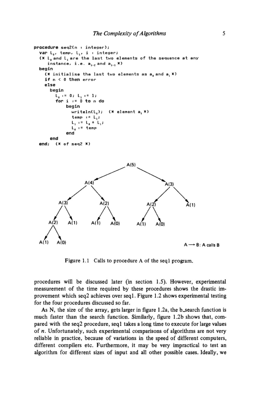
The Complexity of Algorithms 5 procedure seq2(n integer); var Lo,temp,L,i integer; (x L,and L are the last two elements of the sequence at any instance,i.e.a1-2 and a-1x) begin (x initialise the last two elements as a,and a;x) if n 0 then error else begin L。1=0;L14=1: for i :=0 to n do begin writeln(L);(x element a,x) temp :L L1:=L。+L,i L。:=temp end end end;(关of seq2) A(5) A(4) A(3)】 A(3 A(2) A2) A(1) A(1) A(1) A(O) A(1) A(O) A(O A→B:A calls B Figure 1.1 Calls to procedure A of the seql program. procedures will be discussed later (in section 1.5).However,experimental measurement of the time required by these procedures shows the drastic im- provement which seq2 achieves over seq1.Figure 1.2 shows experimental testing for the four procedures discussed so far. As N,the size of the array,gets larger in figure 1.2a,the b_search function is much faster than the search function.Similarly,figure 1.2b shows that,com- pared with the seg2 procedure,seql takes a long time to execute for large values of n.Unfortunately,such experimental comparisons of algorithms are not very reliable in practice,because of variations in the speed of different computers, different compilers etc.Furthermore,it may be very impractical to test an algorithm for different sizes of input and all other possible cases.Ideally,we
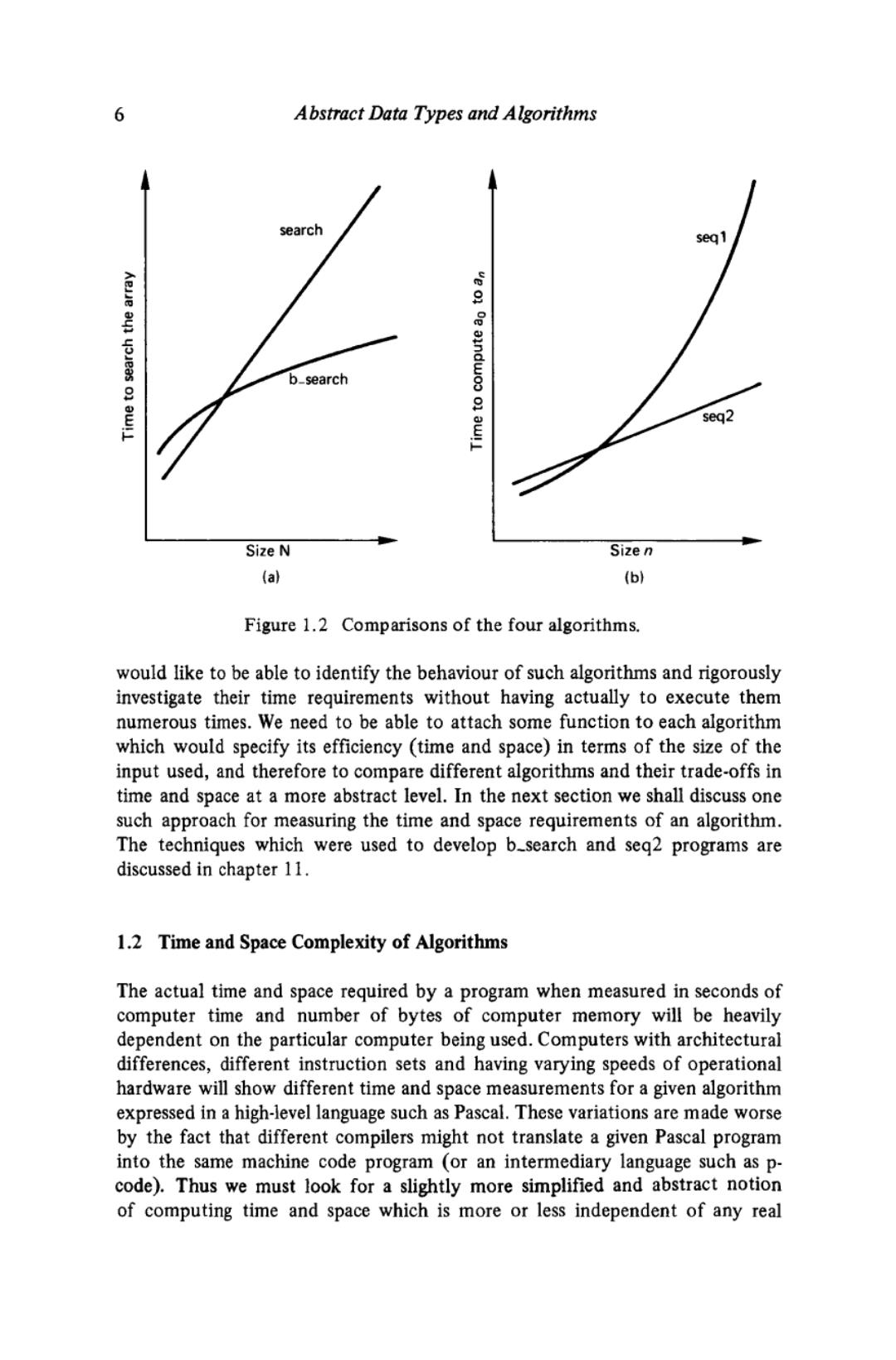
6 Abstract Data Types and Algorithms search seq 1 ve on b_search seq2 Size N Size n (a) (6) Figure 1.2 Comparisons of the four algorithms. would like to be able to identify the behaviour of such algorithms and rigorously investigate their time requirements without having actually to execute them numerous times.We need to be able to attach some function to each algorithm which would specify its efficiency (time and space)in terms of the size of the input used,and therefore to compare different algorithms and their trade-offs in time and space at a more abstract level.In the next section we shall discuss one such approach for measuring the time and space requirements of an algorithm. The techniques which were used to develop b_search and seg2 programs are discussed in chapter 11. 1.2 Time and Space Complexity of Algorithms The actual time and space required by a program when measured in seconds of computer time and number of bytes of computer memory will be heavily dependent on the particular computer being used.Computers with architectural differences,different instruction sets and having varying speeds of operational hardware will show different time and space measurements for a given algorithm expressed in a high-level language such as Pascal.These variations are made worse by the fact that different compilers might not translate a given Pascal program into the same machine code program (or an intermediary language such as p- code).Thus we must look for a slightly more simplified and abstract notion of computing time and space which is more or less independent of any real