230 Solutions to Problems >(2)=G12(0.1,28.3,1.27,0,3) 切= 1.27001.5255 >>(3)=G12(0.2,28.3,1.27,0,3) w= 1.27001.52551.8383 >(4)=G12(0.3,28.3,1.27,0,3) W= 1.27001.52551.83832.2297 >w(5)=G12(0.4,28.3,1.27,0,3) w= 1.27001.52551.83832.22972.7340 >w(6)=G12(0.5,28.3,1.27,0,3) W= 1.27001.52551.83832.22972.73403.4082 >>w(7)=G12(0.6,28.3,1.27,0,3) W= 1.27001.52551.83832.22972.73403.40824.3552 >w(8)=G12(0.7,28.3,1.27,0,3) w= 1.27001.52551.83832.22972.73403.40824.3552 5.7830 >(9)=G12(0.8,28.3,1.27,0,3)
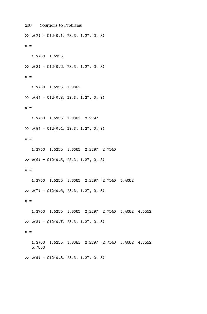
230 Solutions to Problems >> w(2) = G12(0.1, 28.3, 1.27, 0, 3) w = 1.2700 1.5255 >> w(3) = G12(0.2, 28.3, 1.27, 0, 3) w = 1.2700 1.5255 1.8383 >> w(4) = G12(0.3, 28.3, 1.27, 0, 3) w = 1.2700 1.5255 1.8383 2.2297 >> w(5) = G12(0.4, 28.3, 1.27, 0, 3) w = 1.2700 1.5255 1.8383 2.2297 2.7340 >> w(6) = G12(0.5, 28.3, 1.27, 0, 3) w = 1.2700 1.5255 1.8383 2.2297 2.7340 3.4082 >> w(7) = G12(0.6, 28.3, 1.27, 0, 3) w = 1.2700 1.5255 1.8383 2.2297 2.7340 3.4082 4.3552 >> w(8) = G12(0.7, 28.3, 1.27, 0, 3) w = 1.2700 1.5255 1.8383 2.2297 2.7340 3.4082 4.3552 5.7830 >> w(9) = G12(0.8, 28.3, 1.27, 0, 3)
Solutions to Problems 231 W= 1.27001.52551.83832.22972.73403.40824.3552 5.78308.1823 >(10)=G12(0.9,28.3,1.27,0,3) 切= 1.27001.52551.83832.22972.73403.40824.3552 5.78308.182313.0553 >w(11)=G12(1,28.3,1.27,0,3) W= Columns 1 through 10 1.27001.52551.83832.22972.73403.40824.3552 5.78308.182313.0553 Column 11 28.3000 >x=[0;0.1;0.2;0.3;0.4;0.50.6;0.7;0.8; 0.9;1] X= 0 0.1000 0.2000 0.3000 0.4000 0.5000 0.6000 0.7000 0.8000 0.9000 1.0000 >>plot(x,y,k-’,x,z,k-’,x,w,k-.) >x1abe1(‘Vf); >y1abe1(‘G-0120GPa'); >>1 egend(p=1',‘p=2',‘p=3',3);
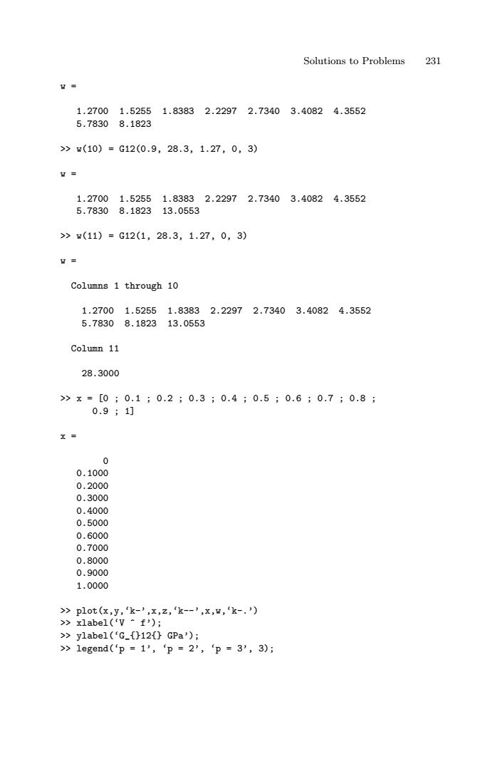
Solutions to Problems 231 w = 1.2700 1.5255 1.8383 2.2297 2.7340 3.4082 4.3552 5.7830 8.1823 >> w(10) = G12(0.9, 28.3, 1.27, 0, 3) w = 1.2700 1.5255 1.8383 2.2297 2.7340 3.4082 4.3552 5.7830 8.1823 13.0553 >> w(11) = G12(1, 28.3, 1.27, 0, 3) w = Columns 1 through 10 1.2700 1.5255 1.8383 2.2297 2.7340 3.4082 4.3552 5.7830 8.1823 13.0553 Column 11 28.3000 >> x = [0 ; 0.1 ; 0.2 ; 0.3 ; 0.4 ; 0.5 ; 0.6 ; 0.7 ; 0.8 ; 0.9 ; 1] x = 0 0.1000 0.2000 0.3000 0.4000 0.5000 0.6000 0.7000 0.8000 0.9000 1.0000 >> plot(x,y,‘k-’,x,z,‘k--’,x,w,‘k-.’) >> xlabel(‘V ^ f’); >> ylabel(‘G_{}12{} GPa’); >> legend(‘p = 1’, ‘p = 2’, ‘p = 3’, 3);

232 Solutions to Problems 30 -p=2 p=3 10 01 02030.405060.70.80.9 Fig.Variation of G12 versus V/for Problem 3.8 Problem 3.9 First,the longitudinal coefficient of thermal expansion a is calculated in /K as follows: >A1pha1(0.6,233,4.62,-0.540e-6,41.4e-6) ans 7.1671e-009 Next,the transverse coefficient of thermal expansion a2 is calculated in /K using two different formulas as follows.Notice that in the second formula,we need to calculate also the value of the longitudinal modulus E.Note also that the two values obtained are comparable and very close to each other. >>A1pha2(0.6,10.10e-6,41.4e-6,0,0,0,0,0,0,1) ans 2.2620e-005 >E1=E1(0.6,233,4.62) E1= 141.6480
232 Solutions to Problems Fig. Variation of G12 versus V f for Problem 3.8 Problem 3.9 First, the longitudinal coefficient of thermal expansion α1 is calculated in /K as follows: >> Alpha1(0.6, 233, 4.62, -0.540e-6, 41.4e-6) ans = 7.1671e-009 Next, the transverse coefficient of thermal expansion α2 is calculated in /K using two different formulas as follows. Notice that in the second formula, we need to calculate also the value of the longitudinal modulus E1. Note also that the two values obtained are comparable and very close to each other. >> Alpha2(0.6, 10.10e-6, 41.4e-6, 0, 0, 0, 0, 0, 0, 1) ans = 2.2620e-005 >> E1 = E1(0.6, 233, 4.62) E1 = 141.6480
Solutions to Problems 233 >>A1pha2(0.6,10.10e-6,41.4e-6,E1,233,4.62,0.200, 0.360,-0.540e-6,2) ans 2.8515e-005 Problem 3.10 E1=E时V于+EmVm+EVi Note that the derivation of the above equation is very similar to the derivation in Example 3.1. Problem 4.1 -V12 51马 01 02 2 T12 0 G12 Problem 4.2 E V12E2 0 1-h221 1-h2'21 12E2 E2 1-221 1-221 Y12 0 0 G12 where v12E2 v21E1. Problem 4.3 IEE 1 0 2(1+v) T12
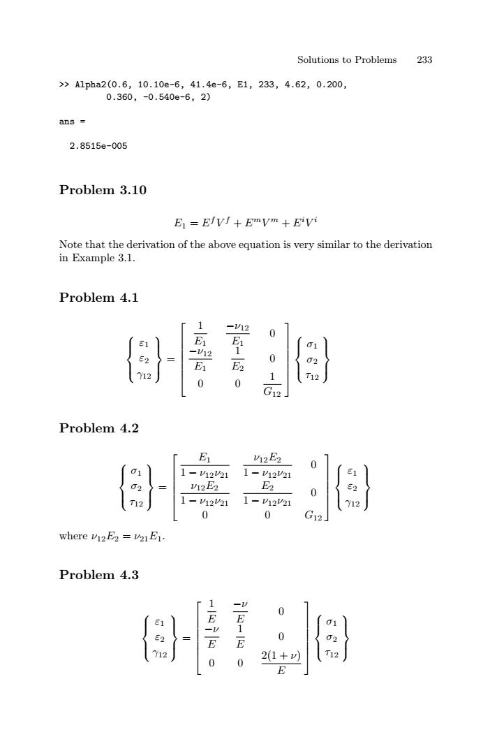
Solutions to Problems 233 >> Alpha2(0.6, 10.10e-6, 41.4e-6, E1, 233, 4.62, 0.200, 0.360, -0.540e-6, 2) ans = 2.8515e-005 Problem 3.10 E1 = EfV f + EmV m + Ei V i Note that the derivation of the above equation is very similar to the derivation in Example 3.1. Problem 4.1 ⎧ ⎪⎨ ⎪⎩ ε1 ε2 γ12 ⎫ ⎪⎬ ⎪⎭ = ⎡ ⎢ ⎢ ⎢ ⎢ ⎢ ⎣ 1 E1 −ν12 E1 0 −ν12 E1 1 E2 0 0 0 1 G12 ⎤ ⎥ ⎥ ⎥ ⎥ ⎥ ⎦ ⎧ ⎪⎨ ⎪⎩ σ1 σ2 τ12 ⎫ ⎪⎬ ⎪⎭ Problem 4.2 ⎧ ⎪⎨ ⎪⎩ σ1 σ2 τ12 ⎫ ⎪⎬ ⎪⎭ = ⎡ ⎢ ⎢ ⎢ ⎢ ⎣ E1 1 − ν12ν21 ν12E2 1 − ν12ν21 0 ν12E2 1 − ν12ν21 E2 1 − ν12ν21 0 0 0 G12 ⎤ ⎥ ⎥ ⎥ ⎥ ⎦ ⎧ ⎪⎨ ⎪⎩ ε1 ε2 γ12 ⎫ ⎪⎬ ⎪⎭ where ν12E2 = ν21E1. Problem 4.3 ⎧ ⎪⎨ ⎪⎩ ε1 ε2 γ12 ⎫ ⎪⎬ ⎪⎭ = ⎡ ⎢ ⎢ ⎢ ⎢ ⎢ ⎣ 1 E −ν E 0 −ν E 1 E 0 0 0 2(1 + ν) E ⎤ ⎥ ⎥ ⎥ ⎥ ⎥ ⎦ ⎧ ⎪⎨ ⎪⎩ σ1 σ2 τ12 ⎫ ⎪⎬ ⎪⎭

234 Solutions to Problems Problem 4.4 E vE 0 01 1-w2 1-v2 E1 vE E 0 1-w2 1-v2 E2 T12 E Y12 0 0 2(1+v)」 Problem 4.5 >>S ReducedCompliance(50.0,15.2,0.254,4.70) S= 0.0200 -0.0051 0 -0.0051 0.0658 0 0 0 0.2128 >>Q=ReducedStiffness(50.0,15.2,0.254,4.70) Q= 51.0003 3.9380 0 3.9380 15.5041 0 0 0 4.7000 >>S*Q ans 1.0000 0 0 0 1.0000 0 0 01.0000 Problem 4.6 >>S=0 rthotropicComp1 iance(155.0,12.10,12.10,0.248,0.458, 0.248,4.40,3.20,4.40) S= 0.0065 -0.0016 -0.0016 0 0 0 -0.0016 0.0826 -0.0379 0 0 0
234 Solutions to Problems Problem 4.4 ⎧ ⎪⎨ ⎪⎩ σ1 σ2 τ12 ⎫ ⎪⎬ ⎪⎭ = ⎡ ⎢ ⎢ ⎢ ⎢ ⎢ ⎣ E 1 − ν2 νE 1 − ν2 0 νE 1 − ν2 E 1 − ν2 0 0 0 E 2(1 + ν) ⎤ ⎥ ⎥ ⎥ ⎥ ⎥ ⎦ ⎧ ⎪⎨ ⎪⎩ ε1 ε2 γ12 ⎫ ⎪⎬ ⎪⎭ Problem 4.5 >> S = ReducedCompliance(50.0, 15.2, 0.254, 4.70) S = 0.0200 -0.0051 0 -0.0051 0.0658 0 0 0 0.2128 >> Q = ReducedStiffness(50.0, 15.2, 0.254, 4.70) Q = 51.0003 3.9380 0 3.9380 15.5041 0 0 0 4.7000 >> S*Q ans = 1.0000 0 0 0 1.0000 0 0 0 1.0000 Problem 4.6 >> S = OrthotropicCompliance(155.0, 12.10, 12.10, 0.248, 0.458, 0.248, 4.40, 3.20, 4.40) S = 0.0065 -0.0016 -0.0016 0 0 0 -0.0016 0.0826 -0.0379 0 0 0