Chapter 3 Random Variables and their Distributions A random variable is a rule or function that assigns numerical values to observations or measurements.It is called a random variable because the number that is assigned to the observation is a numerical event which varies randomly.It can take different values for different observations or measurements of an experiment.A random variable takes a numerical value with some probability. Throughout this book,the symbol y will denote a variable and y will denote a particular val lue of an observation 1.For a particular obs ervation letter 1 be replac with a natural number (v,y2,etc).The symbol yo will denote a particular value,fo example,ysyo will mean that the variable y has all values that are less than or equal to some value yo. Random variables can be discrete or continuous.A continuous variable can take on all values in an interval of real numbers.For example,calf weight at the age of six months might take any possible value in an interval from 10 to 260 kg.s say the value of 180.0 kg kg:hov ales or practical use determi es the number o decimal places he values vill be reported. A discrete variable can take only particula (ofte integ rs)and not all values in some interval.For example,the onth,litter size,etc event and t hus it ha some probabil ility.A table grapn ol proba he prob ability te and ng th we us a m on as or em ru nat pre dis are pres theoretical probability dist continuous variables are called probability density functions 3.1 Expectations and Variances of Random Variables Important parameters describing a random variable are the mean (expectation)and variance.The term expectation is interchangeable with mean,because the expected value of the typical member is the mean.The expectation of a variabley is denoted with: E0)=4 The variance ofy is: Va0y)=o2,=E0y-4,)]1=E62)-4,2 公
26 Chapter 3 Random Variables and their Distributions A random variable is a rule or function that assigns numerical values to observations or measurements. It is called a random variable because the number that is assigned to the observation is a numerical event which varies randomly. It can take different values for different observations or measurements of an experiment. A random variable takes a numerical value with some probability. Throughout this book, the symbol y will denote a variable and yi will denote a particular value of an observation i. For a particular observation letter i will be replaced with a natural number (y1, y2, etc). The symbol y0 will denote a particular value, for example, y ≤ y0 will mean that the variable y has all values that are less than or equal to some value y0. Random variables can be discrete or continuous. A continuous variable can take on all values in an interval of real numbers. For example, calf weight at the age of six months might take any possible value in an interval from 160 to 260 kg, say the value of 180.0 kg or 191.23456 kg; however, precision of scales or practical use determines the number of decimal places to which the values will be reported. A discrete variable can take only particular values (often integers) and not all values in some interval. For example, the number of eggs laid in a month, litter size, etc. The value of a variable y is a numerical event and thus it has some probability. A table, graph or formula that shows that probability is called the probability distribution for the random variable y. For the set of observations that is finite and countable, the probability distribution corresponds to a frequency distribution. Often, in presenting the probability distribution we use a mathematical function as a model of empirical frequency. Functions that present a theoretical probability distribution of discrete variables are called probability functions. Functions that present a theoretical probability distribution of continuous variables are called probability density functions. 3.1 Expectations and Variances of Random Variables Important parameters describing a random variable are the mean (expectation) and variance. The term expectation is interchangeable with mean, because the expected value of the typical member is the mean. The expectation of a variable y is denoted with: E(y) = µy The variance of y is: Var(y) = σ2 y = E[(y – µy) 2 ] = E(y 2 ) – µy 2
Chapter 3 Random Variables and their Distributions 27 which is the mean square deviation from the mean.Recall that the standard deviation is the square root of the variance: There are certain rules that apply when a constant is multiplied or added to a variable,or two variables are added to each other. 1)The expectation of a constant c is the value of the constant itself. E(c)=c 2)The expectation of the sum of a constant c and a variabley is the sum of the constant and expectation of the variable y: E(c+y)=c+E(y) This indicates that when the same number is added to each value of a variable the mean increases by that number 3)The expectation of the product of a constantc and a variableyis equal to the product of the constant and the expectation of the variable y: E(cy)=cE(y) This indicates that if each value of the variable is multiplied by the same number,then the expectation is multiplied by that number. ponof the sum of two variablesandy is the sum of the expectations of the E(x+y)=E(x)+E() 5)The variance of a constant c is equal to zero: Var(c)=0 6)The variance of the product of a constantand a variableyis the product of the squared constant multiplied by the variance of the variabley. Varcy)=cVary) 7)The covariance of two variables x and y: Cox)=Er-4y-4】= =E))-Ex)E0)= =Ey)-4, The covariance is a measure of simultaneous variability of two variables. 8)The variance of the sum of two variables is equal to the sum of the individual variances plus two times the covariance. Var(x+y)=Var(x)+Var(y)+2Cov(xy)
Chapter 3 Random Variables and their Distributions 27 which is the mean square deviation from the mean. Recall that the standard deviation is the square root of the variance: 2 σ = σ There are certain rules that apply when a constant is multiplied or added to a variable, or two variables are added to each other. 1) The expectation of a constant c is the value of the constant itself: E(c) = c 2) The expectation of the sum of a constant c and a variable y is the sum of the constant and expectation of the variable y: E(c + y) = c + E(y) This indicates that when the same number is added to each value of a variable the mean increases by that number. 3) The expectation of the product of a constant c and a variable y is equal to the product of the constant and the expectation of the variable y: E(cy) = cE(y) This indicates that if each value of the variable is multiplied by the same number, then the expectation is multiplied by that number. 4) The expectation of the sum of two variables x and y is the sum of the expectations of the two variables: E(x + y) = E(x) + E(y) 5) The variance of a constant c is equal to zero: Var(c) = 0 6) The variance of the product of a constant c and a variable y is the product of the squared constant multiplied by the variance of the variable y: Var(cy) = c 2 Var(y) 7) The covariance of two variables x and y: Cov(x,y) = E[(x – µx)(y – µy)] = = E(xy) – E(x)E(y) = = E(xy) – µxµy The covariance is a measure of simultaneous variability of two variables. 8) The variance of the sum of two variables is equal to the sum of the individual variances plus two times the covariance: Var(x + y) = Var(x) + Var(y) + 2Cov(x,y)
28 Biostatistics for Animal Science 3.2 Probability Distributions for Discrete Random Variables The probability distribution for a discrete random variable y is the table,graph or formula that assigns the probability P()for each possible value of the variable y.The probability distribution P()must satisfy the following two assumptions: 1)0≤Py≤1 The probability of each value must be between 0 and 1,inclusively. 2)ZnP0)=1 The sum of probabilities of all possible values of a variabley is equal to 1. Example:An ex A ble coin Let Ha nd T denote head and tail. of ads in coins.Possib The events and associated probabilities are shown in the following table The simple events are denoted with E,E2,E and E.There are four possible simple events HH,HT,TH,and IT. Simple event Description y P(y) E. HH 2 4 HT E TH 1 E 0 From the table we can see tha T he prob ility that y =2 2)=PE=4 Ine proba =PE)+PE)=4+h=2 The probability that y=0 is P(y=0)=P(E)= Thus,the probability distribution of the variableyis P(y) 0 2 L Checking the previously stated assumptions 1.0≤P6)≤1 2.∑P0=P0=0)+P0=I)+P心=2)=%+⅓+⅓-
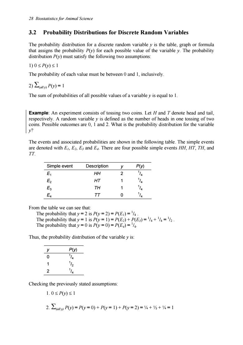
28 Biostatistics for Animal Science 3.2 Probability Distributions for Discrete Random Variables The probability distribution for a discrete random variable y is the table, graph or formula that assigns the probability P(y) for each possible value of the variable y. The probability distribution P(y) must satisfy the following two assumptions: 1) 0 ≤ P(y) ≤ 1 The probability of each value must be between 0 and 1, inclusively. 2) Σ(all y) P(y) = 1 The sum of probabilities of all possible values of a variable y is equal to 1. Example: An experiment consists of tossing two coins. Let H and T denote head and tail, respectively. A random variable y is defined as the number of heads in one tossing of two coins. Possible outcomes are 0, 1 and 2. What is the probability distribution for the variable y? The events and associated probabilities are shown in the following table. The simple events are denoted with E1, E2, E3 and E4. There are four possible simple events HH, HT, TH, and TT. Simple event Description y P(y) E1 HH 2 1 /4 E2 HT 1 1 /4 E3 TH 1 1 /4 E4 TT 0 1 /4 From the table we can see that: The probability that y = 2 is P(y = 2) = P(E1) = 1 /4 . The probability that y = 1 is P(y = 1) = P(E2) + P(E3) = 1 /4 + 1 /4 = 1 /2 . The probability that y = 0 is P(y = 0) = P(E4) = 1 /4. Thus, the probability distribution of the variable y is: y P(y) 0 1 /4 1 1 /2 2 1 /4 Checking the previously stated assumptions: 1. 0 ≤ P(y) ≤ 1 2. Σ(all y) P(y) = P(y = 0) + P(y = 1) + P(y = 2) = ¼ + ½ + ¼ = 1
Chapter 3 Random Variables and their Distributions 29 A cumulative probability distribution F describes the probability that a variableyhas values less than or equal to some value y: FW=POy≤W Example:For the example of tossing two coins,what is the cumulative distribution? We have: P(y)F(y) 0 4 1 2 3 2 For example,the probability F(1)denotes the probability that y.the number of heads, is 0 or 1,that is,in tossing two coins that we have at least one tail (or we do not have two heads). 3.2.1 Expectation and Variance of a Discrete Random Variable The expectation or mean of a discrete variable y is defined: E0=4=∑P0Wy i=1,n The variance of a discrete random variabley is defined: a0)=G2=Ey-Eyj}=∑,P0)y-E0yi=1,n Example:Calculate the expectation and variance of the number of heads resulting from tossing two coins. Expectation: Ey=u=∑,P0)y,=(a)0)+)I)+(a)(2)=1 The expected value is one head and one tail when tossing two coins. Variance: Vay=d2=∑P)y-E0y2=(ha)0-12+(2)(1-1)2+)(2-12=(2)
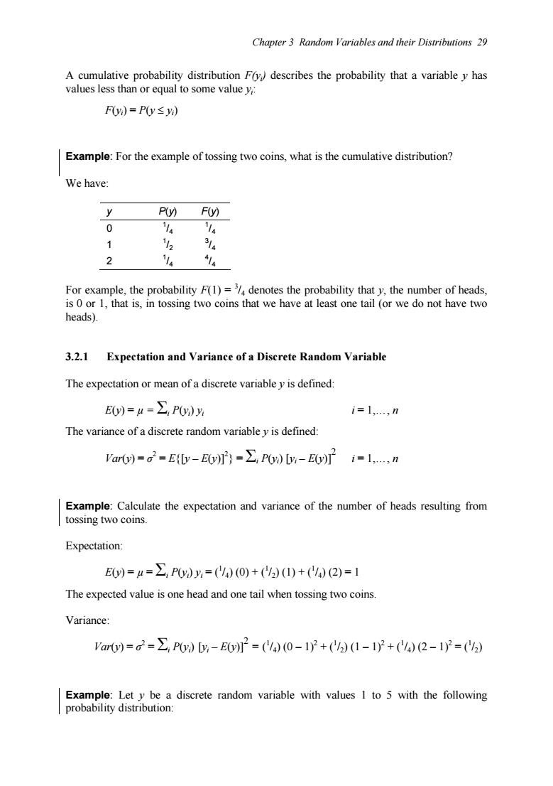
Chapter 3 Random Variables and their Distributions 29 A cumulative probability distribution F(yi) describes the probability that a variable y has values less than or equal to some value yi: F(yi) = P(y ≤ yi) Example: For the example of tossing two coins, what is the cumulative distribution? We have: y P(y) F(y) 0 1 /4 1 /4 1 1 /2 3 /4 2 1 /4 4 /4 For example, the probability F(1) = 3 /4 denotes the probability that y, the number of heads, is 0 or 1, that is, in tossing two coins that we have at least one tail (or we do not have two heads). 3.2.1 Expectation and Variance of a Discrete Random Variable The expectation or mean of a discrete variable y is defined: E(y) = µ = Σi P(yi) yi i = 1,., n The variance of a discrete random variable y is defined: Var(y) = σ2 = E{[y – E(y)]2 } = Σi P(yi) [yi – E(y)]2 i = 1,., n Example: Calculate the expectation and variance of the number of heads resulting from tossing two coins. Expectation: E(y) = µ = Σi P(yi) yi = (1 /4) (0) + (1 /2) (1) + (1 /4) (2) = 1 The expected value is one head and one tail when tossing two coins. Variance: Var(y) = σ2 = Σi P(yi) [yi – E(y)]2 = ( 1 /4) (0 – 1)2 + (1 /2) (1 – 1)2 + (1 /4) (2 – 1)2 = (1 /2) Example: Let y be a discrete random variable with values 1 to 5 with the following probability distribution:
30 Biostatistics for Animal Science 1 2 3 4 5 Frequency 2 4 2 P(y) ho 4/0 Check if the table shows a correct probability distribution.What is the probability thatyis greater than three,P(y>3)? I)0≤Py≤1=OK 2)P0)=1→0K The cumulative frequency ofy=3 is 7. F3)=Py≤3)=P1)+P2)+P3)=(/o)+(o)+(Mo)=(o) Py>3)=P4)+P5)=2,)+ P0>3)=1-P0≤3)= -(1o) Expectation: Ey=u=∑yPy)=(Ho)+(2)1o)+(3)Ho)+(4(Ho)+(5)(Ho)=0o)=3 Variance: ar0=d2=Ey-E0=∑,P0w-E0P= (/o)(1-32+11o)(2-3}+(1o)(3-3)2+1o)(4-32+(1o)(5-3}2=1.2 3.2.2 Bernoulli Distribution 熟am for example Yes and No,or The probability distribution ofy has the Bernoulli distribution p(y)=p'q'fory=0.1 Here,q=1-p Thus, P0y=1)=p P(=0)=q The expectation and variance of a Bernoulli variable are E(v)=u=p and d=Vary)=a=pq
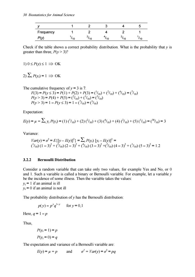
30 Biostatistics for Animal Science y 1 2 3 4 5 Frequency 1 2 4 2 1 P(y) 1 /10 2 /10 4 /10 2 /10 1 /10 Check if the table shows a correct probability distribution. What is the probability that y is greater than three, P(y > 3)? 1) 0 ≤ P(y) ≤ 1 ⇒ OK 2) Σi P(yi) = 1 ⇒ OK The cumulative frequency of y = 3 is 7. F(3) = P(y ≤ 3) = P(1) + P(2) + P(3) = (1 /10) + (2 /10) + (4 /10) = (7 /10) P(y > 3) = P(4) + P(5) = (2 /10) + (1 /10) = (3 /10) P(y > 3) = 1 – P(y ≤ 3) = 1 – (7 /10) = (3 /10) Expectation: E(y) = µ = Σi yi P(yi) = (1) (1 /10) + (2) (2 /10) + (3) (4 /10) + (4) (2 /10) + (5) (1 /10) = (30/10) = 3 Variance: Var(y) = σ2 = E{[y – E(y)]2 } = Σi P(yi) [yi – E(y)]2 = ( 1 /10) (1 – 3)2 + (2 /10) (2 – 3)2 + (4 /10) (3 – 3)2 +(2 /10) (4 – 3)2 + (1 /10) (5 – 3)2 = 1.2 3.2.2 Bernoulli Distribution Consider a random variable that can take only two values, for example Yes and No, or 0 and 1. Such a variable is called a binary or Bernoulli variable. For example, let a variable y be the incidence of some illness. Then the variable takes the values: yi = 1 if an animal is ill yi = 0 if an animal is not ill The probability distribution of y has the Bernoulli distribution: y y p y p q − = 1 ( ) for y = 0,1 Here, q = 1 – p Thus, P(yi = 1) = p P(yi = 0) = q The expectation and variance of a Bernoulli variable are: E(y) = µ = p and σ2 = Var(y) = σ2 = pq