7.2 MATLAB Functions Used 125 025 02 015 005 0 0.05 01 015 025 20 3040 60 o.(MPa) Fig.7.4.Variation of o:versus z for Example 7.1 025 02 05 005 005 -0.15 02 1.5 25 o.(MPa) Fig.7.5.Variation of oy versus z for Example 7.1 The distribution of the stress Try along the depth of the laminate is now plotted as follows (see Fig.7.6): >>x=[sigma4b(3)sigma4a(3)sigma3b(3)sigma3a(3)sigma2b(3)sigma2a(3) sigma1b(3)sigmala(3)] X■ 1.0e-015* 00-0.1162-0.1162-0.1162-0.116200
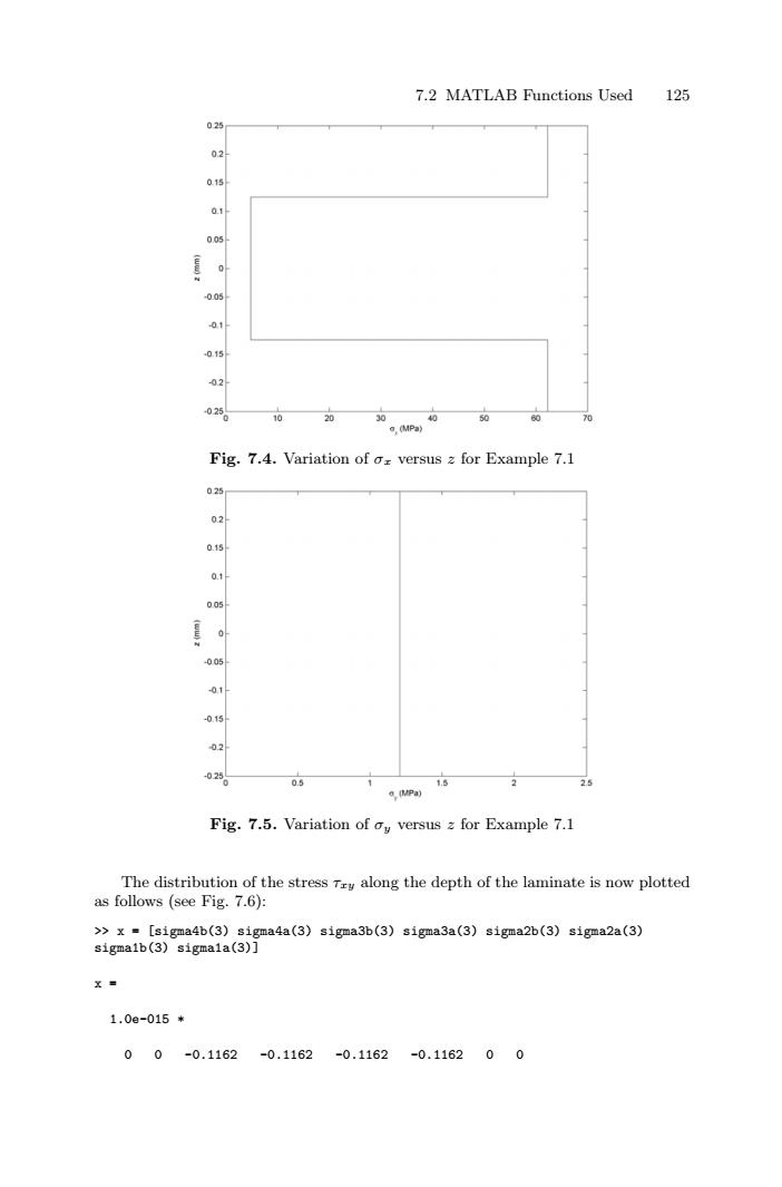
7.2 MATLAB Functions Used 125 Fig. 7.4. Variation of σx versus z for Example 7.1 Fig. 7.5. Variation of σy versus z for Example 7.1 The distribution of the stress τxy along the depth of the laminate is now plotted as follows (see Fig. 7.6): >> x = [sigma4b(3) sigma4a(3) sigma3b(3) sigma3a(3) sigma2b(3) sigma2a(3) sigma1b(3) sigma1a(3)] x = 1.0e-015 * 0 0 -0.1162 -0.1162 -0.1162 -0.1162 0 0
126 7 Laminate Analysis-Part I 025 0,2 015 0.1 005 0.05 0.1 -0.15 02 092 -08 06 0.4 02 t(MPa) g10 Fig.7.6.Variation of Txy versus z for Example 7.1 >plot(x,y) >ylabel(‘z(mm)') >xlabel('\tau_{xy}(MPa)') Next,the three force resultants are calculated in MN/m using (7.13a,b,c)as follows: >Nx =0.125e-3 (sigmala(1)+sigma2a(1)+sigma3a(1)+sigma4a(1)) Nx 0.0168 >Ny =0.125e-3 (sigmala(2)+sigma2a(2)+sigma3a(2)+sigma4a(2)) Ny 6.0306e-004 >Nxy =0.125e-3 (sigmala(3)+sigma2a(3)+sigma3a(3)+sigma4a(3)) Nxy -2.9043e-020 Next,the three moment resultants are calculated in MN.m/m using (7.13d,e,f) as follows:
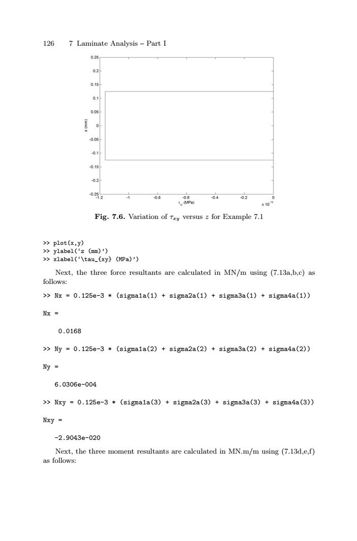
126 7 Laminate Analysis – Part I Fig. 7.6. Variation of τxy versus z for Example 7.1 >> plot(x,y) >> ylabel(‘z (mm)’) >> xlabel(‘\tau_{xy} (MPa)’) Next, the three force resultants are calculated in MN/m using (7.13a,b,c) as follows: >> Nx = 0.125e-3 * (sigma1a(1) + sigma2a(1) + sigma3a(1) + sigma4a(1)) Nx = 0.0168 >> Ny = 0.125e-3 * (sigma1a(2) + sigma2a(2) + sigma3a(2) + sigma4a(2)) Ny = 6.0306e-004 >> Nxy = 0.125e-3 * (sigma1a(3) + sigma2a(3) + sigma3a(3) + sigma4a(3)) Nxy = -2.9043e-020 Next, the three moment resultants are calculated in MN.m/m using (7.13d,e,f) as follows: