11 o-V层[a4e-地={05/an.a if n is even =V()京a受到m2 出oe (田-∑cPEn on of co ation of sP-(F)’-0as… The rest of the coefficients make up the difference 之-(到三 The expectation value of the energy in this example is m-()器-器点-盟 where we have used 品+京+苏+=品 +京+京+…=弱 As one might expeet,it is very close toE-slightly larger,because of the admixture of excited states Problem 2 Griffiths,.5.2.6.(for advanced erercise) IIL.THE HARMONIC OSCILLATOR The classical harmonic oscillator is governed by Hooke's Law F--kr-m
11 cn = √ 2 a ∫ a 0 sin(nπ a x) √ 30 a 5 x(a − x)dx = { 0, if n is even 8 √ 15/ (nπ) 3 , if n is odd Ψ (x, t) = √ 30 a ( 2 π )3 ∑ n=1,3,5··· 1 n3 sin(nπ a x) exp ( −in2π 2 ~t/2ma2 ) Loosely speaking, cn tells you the “amount of ψn that is contained in Ψ”. Some people like to say that |cn| 2 is the “probability of finding the particle in the n-th stationary state”, but this is bad language; the particle is in the state Ψ, not Ψn, and anyhow, in the laboratory you don’t “find a particle to be in a particular state” - you measure some observable, and what you get is a number. As we will see later, what |cn| 2 tells you is the probability that a measurement of the energy would yield the value En. The sum of these probability should be 1, ∑∞ n=1 |cn| 2 = 1, and the expectation value of the energy ⟨H⟩ = ∑∞ n=1 |cn| 2 En is independent of time which is a manifestation of conservation of energy in Quantum Mechanics. The starting wave function closely resembles the ground state ψ1. This suggests that |c1| 2 should dominate, and in fact |c1| 2 = ( 8 √ 15 π 3 )2 = 0.998555 · · · The rest of the coefficients make up the difference ∑∞ n=1 |cn| 2 = ( 8 √ 15 π 3 )2 ∑∞ n=1,3,5··· 1 n6 = 1 The expectation value of the energy in this example is ⟨H⟩ = ∑∞ n=1,3,5··· ( 8 √ 15 π 3 )2 1 n6 n 2π 2~ 2 2ma2 = 480~ 2 π 4ma2 ∑∞ n=1,3,5··· 1 n4 = 5~ 2 ma2 where we have used 1 1 6 + 1 3 6 + 1 5 6 + · · · = π 6 960 1 1 4 + 1 3 4 + 1 5 4 + · · · = π 4 96 As one might expect, it is very close to E1 = π 2~ 2 2ma2 - slightly larger, because of the admixture of excited states. Problem 2 Griffiths, page 38, 2.4, 2.5, 2.6, (for advanced exercise) III. THE HARMONIC OSCILLATOR The classical harmonic oscillator is governed by Hooke’s Law F = −kx = m d 2x dt2
12 FIG.9Parabolic approximation(dashed curve)toan arbitrary potential,in the neighborhood ofa local minimum where m is the mass of the particle and k is the force constant of the spring.The solution is r(t)=Asin(wt)+B cos(wt) with the frequency of oscillation The potential energy is a parabola V回)=kx2 ab the m巴 abolic,in the neighborhood ofa local minimum (Figure).Formally V()=V(ro)+V(zo)(-zo)+jv"(ro)(=-zo)2+... V(e)≌,V"(xoc-xo)2 amplitude is small.The quantum problem is to solve the Schrodinger equation for the potential V(r)=mw2 As we have seen,it suffices to solve the time-independent/stationary equation 器+26- (7) A.Algebraic method:ladder operator To begin with,let's rewrite Equation (7)in a more suggestive form F2+mem月p=Ev because of 品 i=2p2+(mwm)月
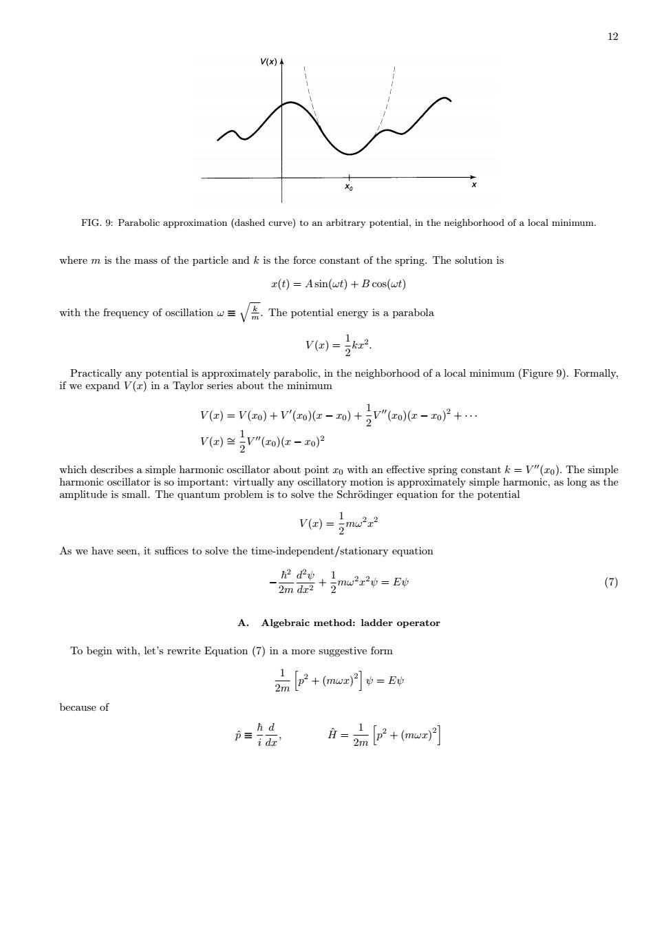
12 FIG. 9: Parabolic approximation (dashed curve) to an arbitrary potential, in the neighborhood of a local minimum. where m is the mass of the particle and k is the force constant of the spring. The solution is x(t) = A sin(ωt) + B cos(ωt) with the frequency of oscillation ω ≡ √ k m . The potential energy is a parabola V (x) = 1 2 kx2 . Practically any potential is approximately parabolic, in the neighborhood of a local minimum (Figure 9). Formally, if we expand V (x) in a Taylor series about the minimum V (x) = V (x0) + V ′ (x0)(x − x0) + 1 2 V ′′(x0)(x − x0) 2 + · · · V (x) ∼= 1 2 V ′′(x0)(x − x0) 2 which describes a simple harmonic oscillator about point x0 with an effective spring constant k = V ′′(x0). The simple harmonic oscillator is so important: virtually any oscillatory motion is approximately simple harmonic, as long as the amplitude is small. The quantum problem is to solve the Schr¨odinger equation for the potential V (x) = 1 2 mω2x 2 As we have seen, it suffices to solve the time-independent/stationary equation − ~ 2 2m d 2ψ dx2 + 1 2 mω2x 2ψ = Eψ (7) A. Algebraic method: ladder operator To begin with, let’s rewrite Equation (7) in a more suggestive form 1 2m [ p 2 + (mωx) 2 ] ψ = Eψ because of pˆ ≡ ~ i d dx, Hˆ = 1 2m [ p 2 + (mωx) 2 ]
13 1.Commutator The idea is to factor the term in square brackets.If these were numbers,it would be casy n2+v2=(u+D)(-iw+) However,uand vare operators and do not commute 筇≠旋 (IfI forget the hat for operators,forgive me).Still this dos motivateus toexamine the quantities a4三2m(年ip+me刘 We see that a-a4=2师+m)(-p+m) =2h(伊+mu-mu-) As anticipated,there is an extra term (p-p),which is called the commutator of and it is a measure of how badly they fail to commute.In general,the commutator of operators A and Bis A.B=AB-BA In this notation, a-a4=2办m+(m门-苏E,月. To figure outwe need give it a test functionf()to act on 压f倒=有0-有f =(毫--)=谢回 Dropping the test function,which has served its purpose [它,创=流 This lovely and ubiquitous result is known as the canonical commutation relation.With this. a=忘i+号 or 且=o(aa,- The Hamiltonian does not factor perfectly-extra term.The ordering of is important a,a.忌- we thus have [a-,a+]=1 and i=加(aa-+) The Schrodinger equationEfor the harmonic oscillator takes the form ne(a4i年±)=E的
13 1. Commutator The idea is to factor the term in square brackets. If these were numbers, it would be easy u 2 + v 2 = (iu + v) (−iu + v) However, u and v are operators and do not commute xˆpˆ ̸= ˆpxˆ (If I forget the hat for operators, forgive me). Still, this does motivate us to examine the quantities aˆ± ≡ 1 √ 2~mω (∓ipˆ+ mωxˆ) We see that aˆ−aˆ+ = 1 2~mω (ipˆ+ mωxˆ) (−ipˆ+ mωxˆ) = 1 2~mω ( pˆ 2 + (mωxˆ) 2 − imω (ˆxpˆ− pˆxˆ) ) As anticipated, there is an extra term (ˆxpˆ− pˆxˆ), which is called the commutator of xˆ and pˆ, it is a measure of how badly they fail to commute. In general, the commutator of operators Aˆ and Bˆ is [ A, ˆ Bˆ ] = AˆBˆ − BˆAˆ In this notation, aˆ−aˆ+ = 1 2~mω [ˆp 2 + (mωxˆ) 2 ] − i 2~ [ˆx, pˆ] . To figure out [ˆx, pˆ], we need give it a test function f(x) to act on [ˆx, pˆ] f(x) = [x ~ i d dx(f) − ~ i d dx(xf)] = ~ i ( x df dx − x df dx − f ) = i~f (x) Dropping the test function, which has served its purpose [ˆx, pˆ] = i~ This lovely and ubiquitous result is known as the canonical commutation relation. With this, aˆ−aˆ+ = 1 ~ω Hˆ + 1 2 or Hˆ = ~ω ( aˆ−aˆ+ − 1 2 ) The Hamiltonian does not factor perfectly - extra term − 1 2 . The ordering of ˆa−aˆ+ is important aˆ+aˆ− = 1 ~ω Hˆ − 1 2 we thus have [ˆa−, aˆ+] = 1 and Hˆ = ~ω ( aˆ+aˆ− + 1 2 ) The Schr¨odinger equation Hψˆ = Eψ for the harmonic oscillator takes the form ~ω ( aˆ±aˆ∓ ± 1 2 ) ψ = Eψ
14 2.Ladder operators Now,here comes the crucial step:I claim that if=E then 户(a+w)=(E+n)(a+9 A(a_)=(E-w)(a-) ia4)=((a4a-+)a+) =hu(a4a_a++5a4) =a+w(a4a-+与+1间 =a+(a+w)p=a+(E+w)p =(E+h)(a4) By the same token,is a solution with energy (E-hw). i(a_)-(E-w)(a_) Bere.theoe foihrfnd ually I'm going to reach a state with energy less a_0=0 ie 2m(径+m)向=0 We can use this to determine o() d =-界 血%=-元r2+omt %=Ae~学 The constant A is given by the normalization 1-wm(←票)-wr =
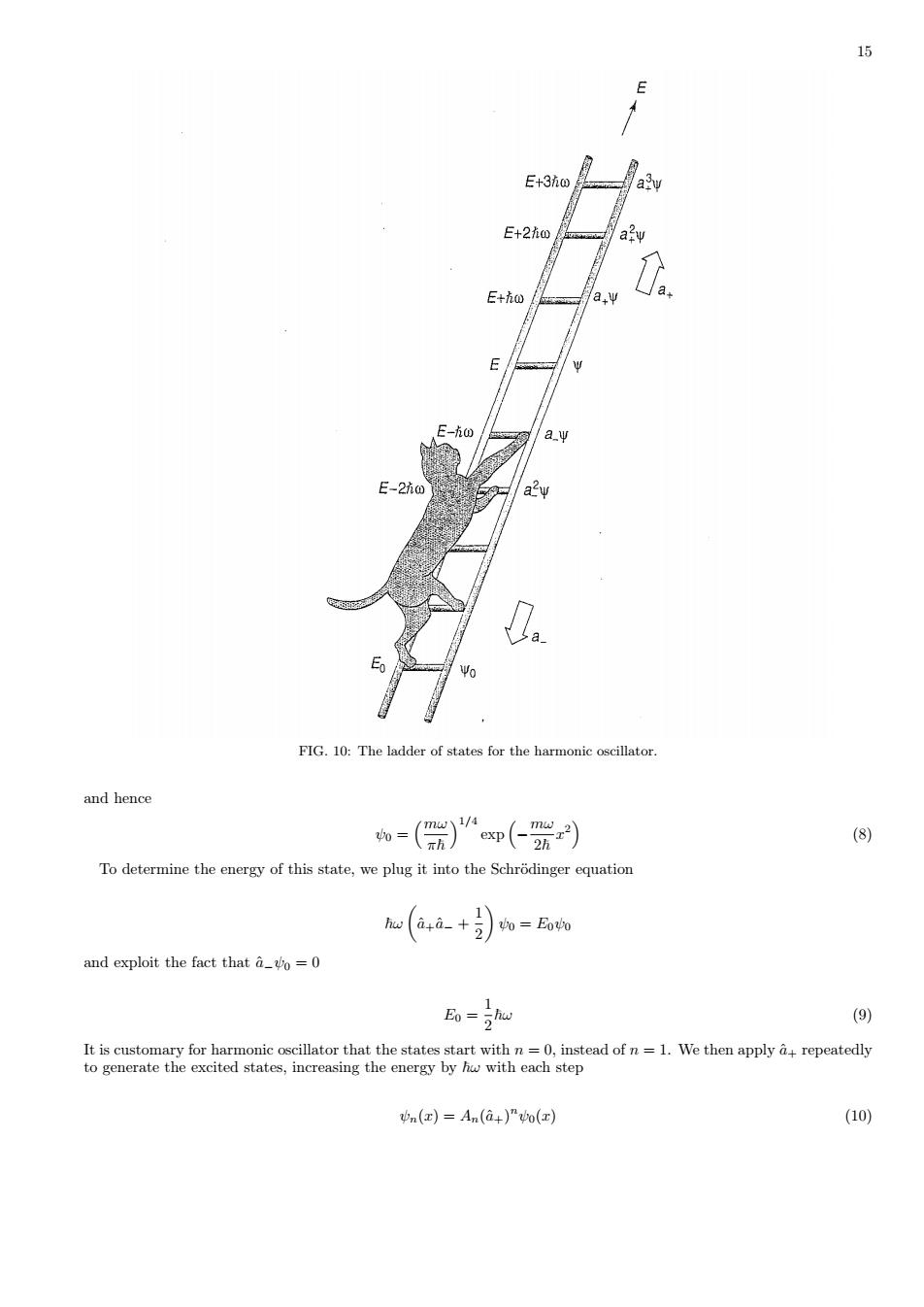
14 2. Ladder operators Now, here comes the crucial step: I claim that if Hψˆ = Eψ then Hˆ (ˆa+ψ) = (E + ~ω) (ˆa+ψ) Hˆ (ˆa−ψ) = (E − ~ω) (ˆa−ψ) Proof: Hˆ (ˆa+ψ) = ~ω ( aˆ+aˆ− + 1 2 ) (ˆa+ψ) = ~ω ( aˆ+aˆ−aˆ+ + 1 2 aˆ+ ) ψ = ˆa+[~ω ( aˆ+aˆ− + 1 2 + 1) ψ] = ˆa+ ( Hˆ + ~ω ) ψ = ˆa+ (E + ~ω) ψ = (E + ~ω) (ˆa+ψ) By the same token, ˆa−ψ is a solution with energy (E − ~ω). Hˆ (ˆa−ψ) = (E − ~ω) (ˆa−ψ) Here, then, is a wonderful machine for generating new solutions, with higher and lower energies - if we could just find one solution, to get started! We call ˆa± ladder operators or raising/lowering operators, because they allow us to climb up and down in energy. The ladder of states is illustrated in Figure 10. But wait! What if I apply the lowering operator repeatedly? Eventually I’m going to reach a state with energy less than zero, which does not exist! At some point the machine must fail. How can that happen? We know that ˆa−ψ is a new solution to the Schr¨odinger equation, but there is no guarantee that it will be normalizable–it might be zero, or its square integral might be infinite. In practice it is the former: There occurs a “lowest rung” (let’s call it ψ0) such that aˆ−ψ0 = 0 i.e 1 √ 2~mω ( ~ d dx + mωx) ψ0 = 0 We can use this to determine ψ0(x) dψ0 dx = − mω ~ xψ0 ∫ dψ0 ψ0 = − mω ~ ∫ xdx ln ψ0 = − mω 2~ x 2 + const. ψ0 = Ae− mω 2~ x 2 The constant A is given by the normalization 1 = |A| 2 ∫ +∞ −∞ exp ( − mω ~ x 2 ) dx = |A| 2 √ ~π mω so A 2 = √ mω π~
15 E E+3i ay E+2h@ E+ho a,Ψ E E-hω aΨ E-2i FIG.10:The ladder of states for the harmonie oscillator. and hence h=()p(←%) (8) To determine the energy of this state,we plug it into the Schrodinger equation @(a4i+》o=Bo and exploit the fact that=0 Eo=hua f=1.We then appa n()=An(a+)严to(a) (10)
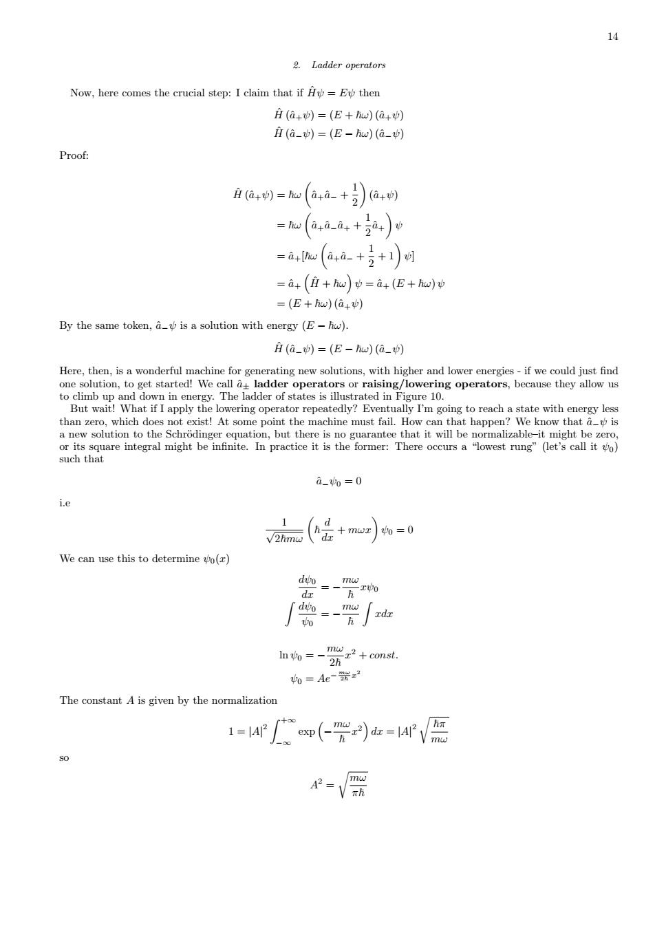
15 FIG. 10: The ladder of states for the harmonic oscillator. and hence ψ0 = (mω π~ )1/4 exp ( − mω 2~ x 2 ) (8) To determine the energy of this state, we plug it into the Schr¨odinger equation ~ω ( aˆ+aˆ− + 1 2 ) ψ0 = E0ψ0 and exploit the fact that ˆa−ψ0 = 0 E0 = 1 2 ~ω (9) It is customary for harmonic oscillator that the states start with n = 0, instead of n = 1. We then apply ˆa+ repeatedly to generate the excited states, increasing the energy by ~ω with each step ψn(x) = An(ˆa+) nψ0(x) (10)