
16 2.When an event can occur in several alternative ways,the probability amplitude for the event is the sum of the probability amplitude for each way considered separately.There is interference: 功=1+ P=+ P=P+P B.Superposition of more than 2 states We have in this case 中=a1%+a2%+…=》a,% al c. state )=cemz+cp (p,t)e'p/h dp which is nothing but the Fourier transformation. C.Measurement of state and probability amplitude 1.Measurement of stat The measurement of state is a rather subtle subject.Let us analyze it as follows: 1.There is a microscopic system in a particular state that is to be measured such as position,momentum,energy,angular momentum,ete. 3.It can be anticipated that the measurement results will be a statistical one. We will discuss here only measurement of two basic physical quantities,the coordinate and the momentum p
16 2. When an event can occur in several alternative ways, the probability amplitude for the event is the sum of the probability amplitude for each way considered separately. There is interference: ψ = ψ1 + ψ2 P = |ψ1 + ψ2| 2 3. If an experiment is performed which is capable of determining whether one or another alternative is actually taken, the probability of the event is the sum of the probabilities for each alternative. The interference is lost: P = P1 + P2 The more precisely you know through which slit the electron passes (particle nature), the more unlikely you will see the interference pattern (wave nature). This is the manifestation of Heisenberg uncertainty principle. B. Superposition of more than 2 states We have in this case ψ = a1ψ1 + a2ψ2 + · · · · · · = ∑ i aiψi where the coefficients ai determine the relative magnitudes and relative phases among the participating waves. A special case, yet the most important one, is the superposition of monochromatic plane waves (with one-dimensional case as example). The superposition of several monochromatic plane waves of different p generates a superposition state ψ(x) = c1e ip1x/~ + c2e ip2x/~ + · · · · · · Generalization: the value p of monochromatic plane wave e ipx/~ changes continuously from −∞ to +∞, the coefficients now are written as a function of p and denoted by φ(p, t) ψ(x, t) = 1 √ 2π~ ∫ +∞ −∞ φ(p, t)e ipx/~ dp which is nothing but the Fourier transformation. C. Measurement of state and probability amplitude 1. Measurement of state The measurement of state is a rather subtle subject. Let us analyze it as follows: 1. There is a microscopic system in a particular state ψ that is to be measured 2. Measurement means that we try to understand the state ψ by means of a process called measurement. This measurement is certainly a macroscopic process and the measured quantity is some kind of physical quantities such as position, momentum, energy, angular momentum, etc. 3. It can be anticipated that the measurement results will be a statistical one. We will discuss here only measurement of two basic physical quantities, the coordinate x and the momentum p
17 W(x) FIG.10:Bragg diffraction element:Different momentum co entsare diffracted into different directions d51n8 dsing FIG.11:Scattering of waves by crystal planes. P(r)dz =v()()dr d.The o the tobe bet()and aliz pointis of finding particle there ot合g是e。)eb,otthep 3.Measurement of momentum iconer the c that the ate)of monochromterbut ()=+e2epzh.… idealized e nt that ca nA 2dsin
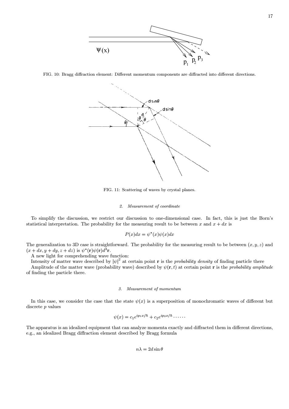
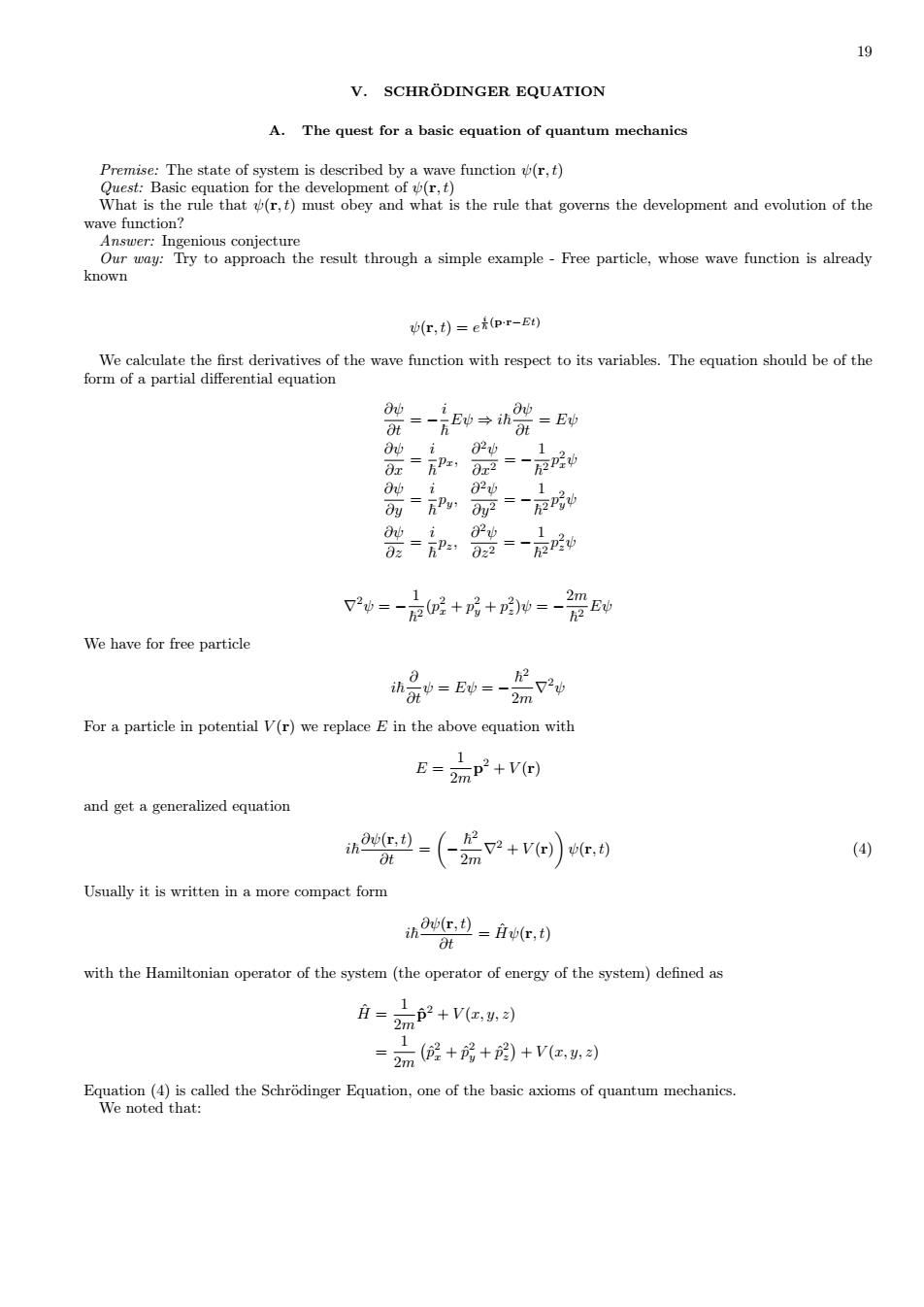
17 p p p1 2 3 ψ(x) FIG. 10: Bragg diffraction element: Different momentum components are diffracted into different directions. FIG. 11: Scattering of waves by crystal planes. 2. Measurement of coordinate To simplify the discussion, we restrict our discussion to one-dimensional case. In fact, this is just the Born’s statistical interpretation. The probability for the measuring result to be between x and x + dx is P(x)dx = ψ ∗ (x)ψ(x)dx The generalization to 3D case is straightforward. The probability for the measuring result to be between (x, y, z) and (x + dx, y + dy, z + dz) is ψ ∗ (r)ψ(r)d 3 r. A new light for comprehending wave function: Intensity of matter wave described by |ψ| 2 at certain point r is the probability density of finding particle there Amplitude of the matter wave (probability wave) described by ψ(r, t) at certain point r is the probability amplitude of finding the particle there. 3. Measurement of momentum In this case, we consider the case that the state ψ(x) is a superposition of monochromatic waves of different but discrete p values ψ(x) = c1e ip1x/~ + c2e ip2x/~ · · · · · · The apparatus is an idealized equipment that can analyze momenta exactly and diffracted them in different directions, e.g., an idealized Bragg diffraction element described by Bragg formula nλ = 2d sin θ

18 The probability for the outcome ofp is proportional to the intensity of the i-th component Generalizing to arbitrary ID state with continuous p values we have 红,0=V2ap,0et中 1 P(p)dp=(p.t)o(p.t)dp=l(p.t)dp Further generalization to 3D case and the probability for the particle to have its momentum between(p)and (p+dp+dp+dp)is P(p)d'p=(p.t)p(p,t)dpadpydp: .Once the w representation of the same state. D.Expectation value of dynamical quantity =pe, =w在,(-h品)e0 and the angular momentum is L=rxp Qe》=eeQ(g-h品)pe利 3) Extension to 3D case is straightforward. significance in quantum theory.We also notice the importance of cartesian coordinate in establishing operator system
18 The probability for the outcome of p is proportional to the intensity of the i−th component c ∗ i ci = |ci | 2 . Generalizing to arbitrary 1D state with continuous p values we have ψ(x, t) = 1 √ 2π~ ∫ φ(p, t)e i ~ pxdp where φ(p, t) plays the role of coefficients ci in the case of continuous p. Hence the probability of finding the particle to have its momentum between p and p + dp P(p)dp = φ ∗ (p, t)φ(p, t)dp = |φ(p, t)| 2 dp Further generalization to 3D case ψ(r, t) = 1 (2π~) 3/2 ∫∫∫ φ(p, t)e i ~ p·r d 3p and the probability for the particle to have its momentum between (px, py, pz) and (px + dpx, py + dpy, pz + dpz) is P(p)d 3p = φ ∗ (p, t)φ(p, t)dpxdpydpz This can be visualized in momentum space as the probability of p vector to have its endpoint in volume element d 3p. Note: • Once the wave function ψ(r, t) is known, φ(p, t) is uniquely defined though Fourier transformation. Thus, the probability distribution of p is known. • ψ(r, t) and φ(p, t) have the same function in representing a state in this sense, i.e., there is no priority of ψ(r, t) over φ(p, t), ψ(r, t) is called coordinate representation of the state, while φ(p, t) is called the momentum representation of the same state. • Just as in coordinate representation, φ(p, t) represents a probability wave and the numerical value of φ(p, t) is the probability amplitude at momentum p. D. Expectation value of dynamical quantity In 1D case we say that the operator x represents position, and the operator −i~ ∂ ∂x represents momentum, in quantum mechanics; to calculate expectation values, we sandwich the appropriate operator between ψ ∗ and ψ, and integrate ⟨x⟩ = ∫ +∞ −∞ dxψ∗ (x, t) (x) ψ (x, t) ⟨px⟩ = ∫ +∞ −∞ dxψ∗ (x, t) ( −i~ ∂ ∂x) ψ (x, t) That’s cute, but what about other dynamical variables? The fact is, all such quantities can be written in terms of position and momentum. Kinetic energy, for example, is T = 1 2 mv2 = p 2 2m and the angular momentum is L = r × p (the latter, of course, does not occur for motion in one dimension). To calculate the expectation value of any such quantity, Q (x, p), we simply replace every p by −i~ ∂ ∂x , insert the resulting operator between ψ ∗ and ψ, and integrate ⟨Q (x, p)⟩ = ∫ +∞ −∞ dxψ∗ (x, t) Q ( x, −i~ ∂ ∂x) ψ (x, t) (3) Extension to 3D case is straightforward. There are two cornerstones of Quantum Mechanics: The state of motion is described by wave functions while dynamical quantities are represented as operators. They cooperate each other into a complete theory. Thus all physical quantities must be operatorized. The consequences of operatorization of physical quantities have profound significance in quantum theory. We also notice the importance of cartesian coordinate in establishing operator system
19 V.SCHRODINGER EQUATION A.The quest for a basic equation of quantum mechanics Premise:The state of system is described by a wave function r,t) wave function? known v(r,t)=e(p-r-E) of the wave function with respect to its variables.The equation should be of the =-E0→h=E -器 光=熟,器=点 2=-京候+居+帅=-祭E的 We have for free particle 哈=v=-品 For a particle in potential V(r)we replace Ein the above equation with E=P+V四 1 and get a generalized equation h2=(编2+vec. () Usually it is written in a more compact form h心c边=ic,) t with the Hamiltonian operator of the system(the operator of energy of the system)defined as i=p2+vg =2房+房+的+V习 end heoodhe ade
19 V. SCHRODINGER EQUATION ¨ A. The quest for a basic equation of quantum mechanics Premise: The state of system is described by a wave function ψ(r, t) Quest: Basic equation for the development of ψ(r, t) What is the rule that ψ(r, t) must obey and what is the rule that governs the development and evolution of the wave function? Answer: Ingenious conjecture Our way: Try to approach the result through a simple example - Free particle, whose wave function is already known ψ(r, t) = e i ~ (p·r−Et) We calculate the first derivatives of the wave function with respect to its variables. The equation should be of the form of a partial differential equation ∂ψ ∂t = − i ~ Eψ ⇒ i~ ∂ψ ∂t = Eψ ∂ψ ∂x = i ~ px, ∂ 2ψ ∂x2 = − 1 ~ 2 p 2 xψ ∂ψ ∂y = i ~ py, ∂ 2ψ ∂y2 = − 1 ~ 2 p 2 yψ ∂ψ ∂z = i ~ pz, ∂ 2ψ ∂z2 = − 1 ~ 2 p 2 zψ ∇2ψ = − 1 ~ 2 (p 2 x + p 2 y + p 2 z )ψ = − 2m ~ 2 Eψ We have for free particle i~ ∂ ∂tψ = Eψ = − ~ 2 2m ∇2ψ For a particle in potential V (r) we replace E in the above equation with E = 1 2m p 2 + V (r) and get a generalized equation i~ ∂ψ(r, t) ∂t = ( − ~ 2 2m ∇2 + V (r) ) ψ(r, t) (4) Usually it is written in a more compact form i~ ∂ψ(r, t) ∂t = Hψˆ (r, t) with the Hamiltonian operator of the system (the operator of energy of the system) defined as Hˆ = 1 2m ˆp 2 + V (x, y, z) = 1 2m ( pˆ 2 x + ˆp 2 y + ˆp 2 z ) + V (x, y, z) Equation (4) is called the Schr¨odinger Equation, one of the basic axioms of quantum mechanics. We noted that:
20 .The Schrodinger equation (4)is not deduced,but conjectured.Its correctness is qualified by the accordance of results deduced from it with experimental facts. .Notice the special ro played by Cartesian coordiate system in obtaining the Hamiltonian .The discussion can be generalized directly to many-body system ih品e,…)=e,…) i=∑2+vn,,…+∑0r) where U()characterize the interaction between particles B.Probability current and probability conservation ha心-(←2+v0 -h-(元2+o) ecan calculate the time derivative of the probability density 层oe-号ow-e =--w An integration over a volume V gives 号l=-会-ep-wa which can be transferred into an integration over the surfacesenclosed by V 层瓜en-品e-血 and 盖er+(a)ew-e=0 Define now the current density of probability as j-(热)-w) we thus arrive at the contination equation of probability density 品f以e,r+f打s-0 架+j=0 盖ne=-fi
20 • The Schr¨odinger equation (4) is not deduced, but conjectured. Its correctness is qualified by the accordance of results deduced from it with experimental facts. • Notice the special role played by Cartesian coordinate system in obtaining the Hamiltonian. • The discussion can be generalized directly to many-body system i~ ∂ ∂tψ (r1, r2, r3, · · ·) = Hψˆ (r1, r2, r3, · · ·) Hˆ = ∑ i 1 2mi ˆp 2 i + V (r1, r2, r3, · · ·) +∑ ij U(rij ) where U(rij ) characterize the interaction between particles. B. Probability current and probability conservation The physical meaning of ρ(r, t) = ψ ∗ (r, t)ψ(r, t) is the probability density. From the Schr¨odinger equation (4) and its complex conjugate i~ ∂ψ(r, t) ∂t = ( − ~ 2 2m ∇2 + V (r) ) ψ(r, t) −i~ ∂ψ∗ (r, t) ∂t = ( − ~ 2 2m ∇2 + V (r) ) ψ ∗ (r, t) we can calculate the time derivative of the probability density i~ ∂ ∂t (ψ ∗ (r, t)ψ(r, t)) = − ~ 2 2m (ψ ∗∇2ψ − ψ∇2ψ ∗ ) = − ~ 2 2m ∇ · (ψ ∗∇ψ − ψ∇ψ ∗ ) An integration over a volume V gives i~ d dt ∫∫∫ V ρ(r, t)d 3 r = − ~ 2 2m ∫∫∫ V ∇ · (ψ ∗∇ψ − ψ∇ψ ∗ )d 3 r which can be transferred into an integration over the surface s enclosed by V i~ d dt ∫∫∫ V ρ(r, t)d 3 r = − ~ 2 2m I s (ψ ∗∇ψ − ψ∇ψ ∗ ) · ds and d dt ∫∫∫ V ρ(r, t)d 3 r + I s ( − i~ 2m ) (ψ ∗∇ψ − ψ∇ψ ∗ ) · ds = 0 Define now the current density of probability as j = ( − i~ 2m ) (ψ ∗∇ψ − ψ∇ψ ∗ ) we thus arrive at the continuation equation of probability density d dt ∫∫∫ V ρ(r, t)d 3 r + I j · ds = 0 and the differential and integral equation of probability conservation ∂ρ ∂t + ∇ · j = 0 d dt ∫∫∫ V ρ(r, t)d 3 r = − I j · ds