Electro in the p A sing FIG.3:Electromagnetic Wave Propagation. o-amplitudemechanical displacement msity U哈→energy density 。Wave function 红,)=Ae(学-2)=Aetm-B Scalar wave.Amplitude-A-? Intensity-AP→ B.Wave packet-a possible way out? Two examples of localized wave packets .Superposition of waves with wave number between (o-Ak)and (+k)-square packet 因={A-AK<+as elsewhere =左 宏24恤a包 工 Amplitude Both wave number and spatial position have a spread-uncertainty relation △xπ/△k △x·△k≈T △r△p≈rh
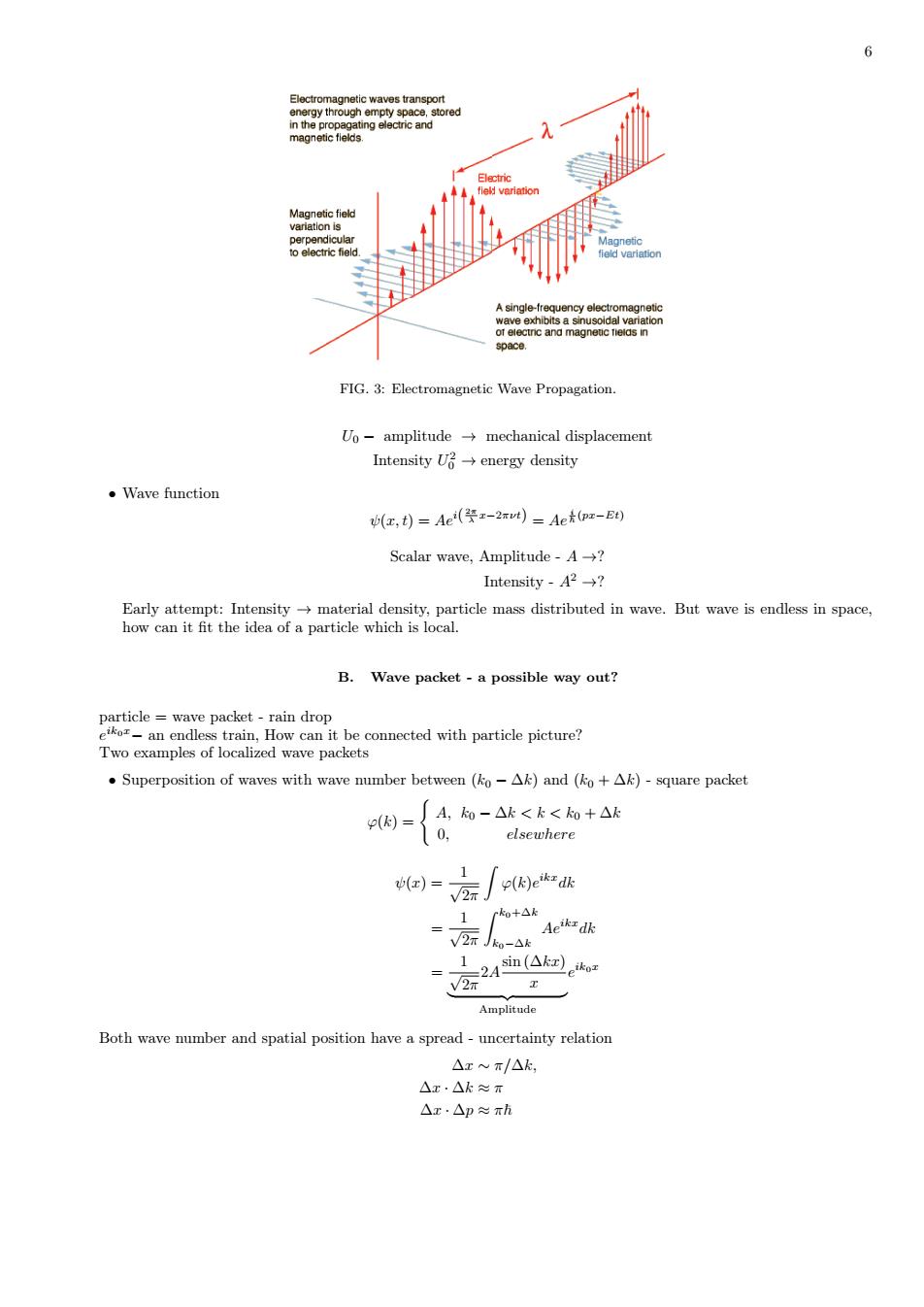
6 FIG. 3: Electromagnetic Wave Propagation. U0 − amplitude → mechanical displacement Intensity U 2 0 → energy density • Wave function ψ(x, t) = Aei( 2π λ x−2πνt) = Ae i ~ (px−Et) Scalar wave, Amplitude - A →? Intensity - A 2 →? Early attempt: Intensity → material density, particle mass distributed in wave. But wave is endless in space, how can it fit the idea of a particle which is local. B. Wave packet - a possible way out? particle = wave packet - rain drop e ik0x− an endless train, How can it be connected with particle picture? Two examples of localized wave packets • Superposition of waves with wave number between (k0 − ∆k) and (k0 + ∆k) - square packet φ(k) = { A, k0 − ∆k < k < k0 + ∆k 0, elsewhere ψ(x) = 1 √ 2π ∫ φ(k)e ikxdk = 1 √ 2π ∫ k0+∆k k0−∆k Aeikxdk = 1 √ 2π 2A sin (∆kx) x | {z } Amplitude e ik0x Both wave number and spatial position have a spread - uncertainty relation ∆x ∼ π/∆k, ∆x · ∆k ≈ π ∆x · ∆p ≈ π~

M 1ANMM AAAAAN W A∧V A水AX1 IG.4:Wave packet formed by plane waves with different frequency Plane wave:elk /ave packet:ko and FIG.5:Spread of a wave packet .Superposition of waves with wave number in a Gaussian packet 2因=(e)e-a- Problem 1 The fou n It is the best Problem:Wave packet is But electros are localized in the atom (1).This viewpont e the e even in enatreaf cro-partic ea ave is cor C.Born's statistical interpretation function,which says that in ID asegives the probability of finding the particle at point at timetor more precisely Probability of findin between a al nd b.at tm
7 FIG. 4: Wave packet formed by plane waves with different frequency. FIG. 5: Spread of a wave packet. • Superposition of waves with wave number in a Gaussian packet φ(k) = ( 2α π )1/4 e −α(k−k0) 2 Problem 1 The Fourier transformation of φ(k) is also Gaussian. It is the best one can do to localize a particle in position and momentum spaces at the same time. Find the root mean square (RMS) deviation ∆x · ∆p =? Problem: Wave packet is unstable - The waves have different phase velocity and the wave components of a wave packet will disperse even in vacuum. But electrons are localized in the atom (1A˚). This viewpoint emphasize the wave nature of micro-particle while killing its particle nature. Another extreme viewpoint on wave particle duality is that wave is composed by large amount of particles (as waves in air). However experiments show clearly a single electron possesses wave nature. This viewpoint over-stressed the particle nature. C. Born’s statistical interpretation A particle by its nature is localized at a point, whereas the wave function is spread out in space. How can such an object represent the state of a particle? The answer is provided by Born’s Statistical Interpretation of the wave function, which says that in 1D case |ψ (x, t)| 2 gives the probability of finding the particle at point x, at time t - or, more precisely ∫ b a |ψ (x, t)| 2 dx = { Probability of finding the particle between a and b, at time t. }
◇ 1011121314151617161920212232425267 FIG.6:Histogram for the distribution etyfor the partice apperingn vome mentoprtiono the intnity Prob ility amplitud dxlw(,3F-(,t)p(,)7 Probability density D.Probability Bec use of the statistical interpretation,probability plays acentral role quantum mechanics.So we introduce ome notation and terminology. 14 people in a room.Let N(j)represent the number of people of age j. N(14)=1,N(15)=1,N(16)=3,N(22)=2,N(24)=2,V(25)=5 while N(17)for instance,is zero.The total number of people in the room is Questions about the distribution this particular age.In general the probability of getting age jis PG)-NU) PG)=1 0 2.What is the most probable age?Answer:25.In general the most probable j is the j for which P()is a maximum. getting a smaller result
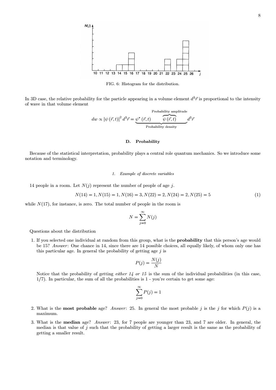
8 FIG. 6: Histogram for the distribution. In 3D case, the relative probability for the particle appearing in a volume element d 3⃗r is proportional to the intensity of wave in that volume element dw ∝ |ψ (⃗r, t)| 2 d 3 ⃗r = ψ ∗ (⃗r, t) Probability amplitude z }| { ψ (⃗r, t) | {z } Probability density d 3 ⃗r D. Probability Because of the statistical interpretation, probability plays a central role quantum mechanics. So we introduce some notation and terminology. 1. Example of discrete variables 14 people in a room. Let N(j) represent the number of people of age j. N(14) = 1, N(15) = 1, N(16) = 3, N(22) = 2, N(24) = 2, N(25) = 5 (1) while N(17), for instance, is zero. The total number of people in the room is N = ∑∞ j=0 N(j) Questions about the distribution 1. If you selected one individual at random from this group, what is the probability that this person’s age would be 15? Answer : One chance in 14, since there are 14 possible choices, all equally likely, of whom only one has this particular age. In general the probability of getting age j is P(j) = N(j) N Notice that the probability of getting either 14 or 15 is the sum of the individual probabilities (in this case, 1/7). In particular, the sum of all the probabilities is 1 - you’re certain to get some age: ∑∞ j=0 P(j) = 1 2. What is the most probable age? Answer : 25. In general the most probable j is the j for which P(j) is a maximum. 3. What is the median age? Answer : 23, for 7 people are younger than 23, and 7 are older. In general, the median is that value of j such that the probability of getting a larger result is the same as the probability of getting a smaller result

FIG.7:Two histogram with different. 4.What is the average(or mean)age?Answer: 国++300+2@+2e+5四-警-21 14 In general the average value ofj(which we shall write thus:())is 6)=2N0-2PU 1=0 a nechanics it is called the expectation value.Nevertheless the yalue is not sgay9器seew 的=2PU) In general,the average value of some function of j is given by U6》-立f6PU j= Beware(2〉≠)2 o三/(a)2〉=VG)-02 △j=j- For the two distributions in the above figure,we have 1=V25.2-25-V0.2 2=V31.0-25=v6 Erample of riables It is simple enough to generalize to continuous distribution.Technically we need "infinitesimal intervals".Thus =p(r)dr
9 FIG. 7: Two histogram with different σ. 4. What is the average (or mean) age? Answer: (14) + (15) + 3 (16) + 2 (22) + 2 (24) + 5 (25) 14 = 294 14 = 21 In general the average value of j (which we shall write thus: ⟨j⟩) is ⟨j⟩ = ∑jN(j) N = ∑∞ j=0 jP(j) In quantum mechanics it is called the expectation value. Nevertheless the value is not necessarily the one you can expect if you made a single measurement. In the above example, you will never get 21. 5. What is the average of the squares of the ages? Answer: You could get 142 = 196, with probability 1/14, or 152 = 225, with probability 1/14, or 162 = 256, with probability 3/14, and so on. The average is ⟨ j 2 ⟩ = ∑∞ j=0 j 2P(j) In general, the average value of some function of j is given by ⟨f(j)⟩ = ∑∞ j=0 f(j)P(j) Beware ⟨ j 2 ⟩ ̸= ⟨j⟩ 2 . Now, there is a conspicuous difference between the following two histograms, even though they have the same median, the same average, the same most probable value, and the same number of elements: The first is sharply peaked about the average value, whereas the second is broad and flat. (The first might represent the age profile for students in a big-city classroom, and the second, perhaps, a rural one-room schoolhouse.) We need a numerical measure of the amount of ”spread” in a distribution, with respect to the average. The most effective way to do this is compute a quantity known as the standard deviation of the distribution σ ≡ √⟨ (∆j) 2 ⟩ = √ ⟨j 2⟩ − ⟨j⟩ 2 ∆j = j − ⟨j⟩ For the two distributions in the above figure, we have σ1 = √ 25.2 − 25 = √ 0.2 σ2 = √ 31.0 − 25 = √ 6 2. Example of continuous variables It is simple enough to generalize to continuous distribution. Technically we need ”infinitesimal intervals”. Thus { Probability that an individual (chosen at random) lies between x and (x + dx) } = ρ(x)dx

10 h FIG.:The probability density in the Examplep() 2点水Temh:bt and6ae Pu=de)de and the ruleswe deduced for discrete distributions translate in the obvious way: (回=xpe)da Uen=CIee达 a2=(△x〉-x)-2 it falls:i distance ut beeth Inongin he distancetime e time near the top,so the average x0=)9t2 片e共 要-√景=后“ Evidently the probability density is 网-2症0≤rs) 1 。2后-a(n0-1
10 FIG. 8: The probability density in the Example ρ(x). ρ(x) is the probability of getting x, or probability density. The probability that x lies between a and b (a finite interval) is given by the integral of ρ(x) Pab = ∫ b a ρ(x)dx and the rules we deduced for discrete distributions translate in the obvious way: 1 = ∫ +∞ −∞ ρ(x)dx ⟨x⟩ = ∫ +∞ −∞ xρ(x)dx ⟨f(x)⟩ = ∫ +∞ −∞ f(x)ρ(x)dx σ 2 ≡ ⟨ (∆x) 2 ⟩ = ⟨ x 2 ⟩ − ⟨x⟩ 2 Example: Suppose I drop a rock off a cliff of height h. As it falls, I snap a million photographs, at random intervals. On each picture I measure the distance the rock has fallen. Question: What is the average of all these distance? That is to say, what is the time average of the distance traveled? Solution: The rock starts out at rest, and picks up speed as it falls; it spends more time near the top, so the average distance must be less than h/2. Ignoring air resistance, the distance x at time t is x(t) = 1 2 gt2 The velocity is dx/dt = gt, and the total flight time is T = √ 2h/g. The probability that the camera flashes in the interval dt is dt/T, so the probability that a given photograph shows a distance in the corresponding range dx is dt T = dx gt √ g 2h = 1 2 √ hx dx Evidently the probability density is ρ(x) = 1 2 √ hx ,(0 ≤ x ≤ h) (outside this range, of course, the probability density is zero.) We can check the normalization of this result ∫ h 0 1 2 √ hx dx = 1 2 √ h ( 2x 1/2 )h 0 = 1