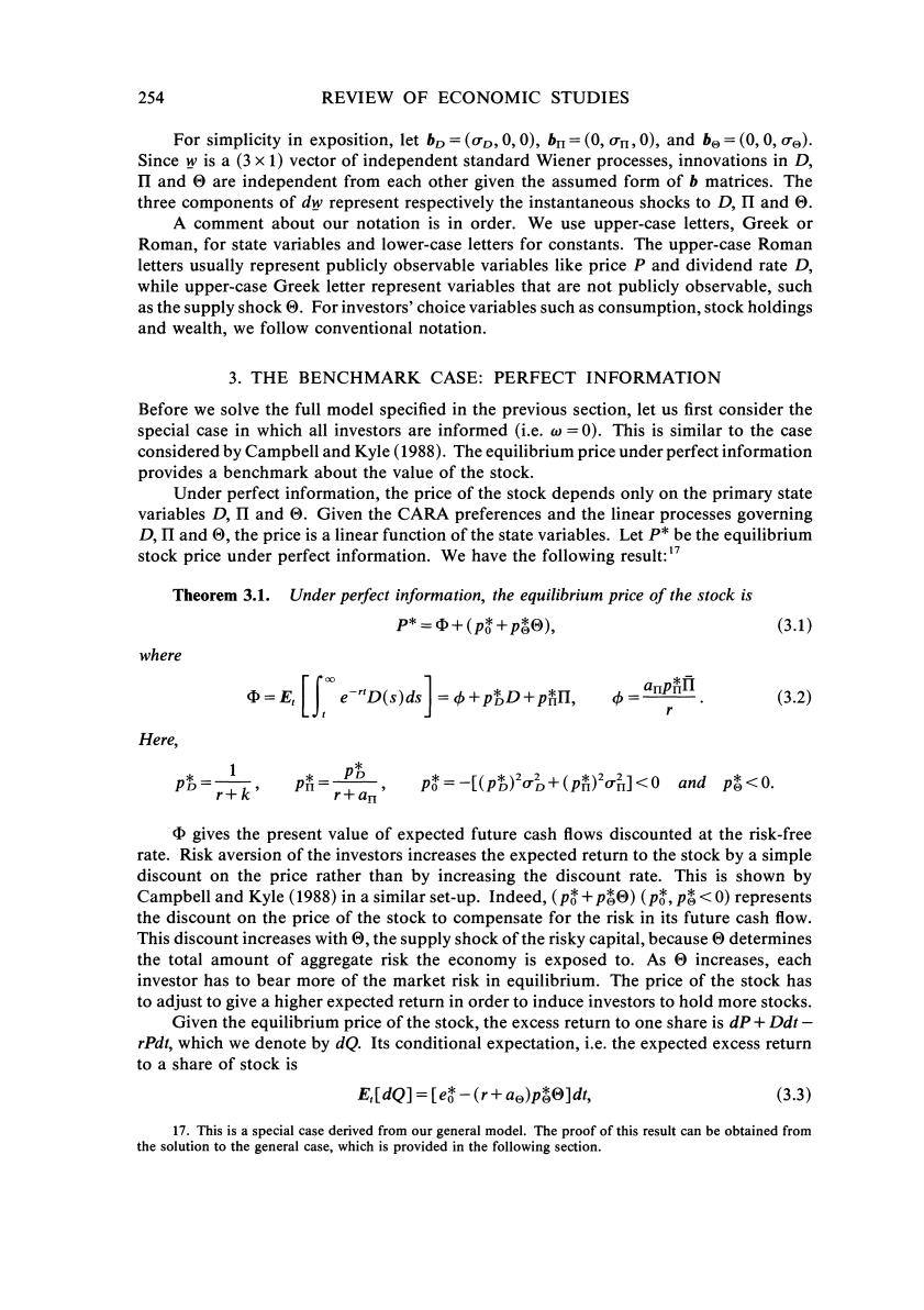
254 REVIEW OF ECONOMIC STUDIES For simplicity in exposition,let bp=(op,0,0),bn=(0,on,0),and be=(0,0,e). Since w is a(3 x 1)vector of independent standard Wiener processes,innovations in D, II and are independent from each other given the assumed form of b matrices.The three components of dw represent respectively the instantaneous shocks to D,II and A comment about our notation is in order.We use upper-case letters,Greek or Roman,for state variables and lower-case letters for constants.The upper-case Roman letters usually represent publicly observable variables like price P and dividend rate D, while upper-case Greek letter represent variables that are not publicly observable,such as the supply shock For investors'choice variables such as consumption,stock holdings and wealth,we follow conventional notation. 3.THE BENCHMARK CASE:PERFECT INFORMATION Before we solve the full model specified in the previous section,let us first consider the special case in which all investors are informed (i.e.@=0).This is similar to the case considered by Campbell and Kyle(1988).The equilibrium price under perfect information provides a benchmark about the value of the stock. Under perfect information,the price of the stock depends only on the primary state variables D,II and Given the CARA preferences and the linear processes governing D,II and the price is a linear function of the state variables.Let P*be the equilibrium stock price under perfect information.We have the following result:7 Theorem 3.1.Under perfect information,the equilibrium price of the stock is P*=中+(p+pΘ), (3.1) where e-"D(s)ds =中+pD+pΠ, =anpin (3.2) Here, r十k, p嘴-p喽 r+an p*=-[(p)2ob+(p)2oi]<0andp<0. gives the present value of expected future cash fows discounted at the risk-free rate.Risk aversion of the investors increases the expected return to the stock by a simple discount on the price rather than by increasing the discount rate.This is shown by Campbell and Kyle(1988)in a similar set-up.Indeed,(p+p)(p,p)represents the discount on the price of the stock to compensate for the risk in its future cash flow. This discount increases with the supply shock of the risky capital,because determines the total amount of aggregate risk the economy is exposed to.As increases,each investor has to bear more of the market risk in equilibrium.The price of the stock has to adjust to give a higher expected return in order to induce investors to hold more stocks. Given the equilibrium price of the stock,the excess return to one share is dp+Ddt- rPdt,which we denote by dQ.Its conditional expectation,i.e.the expected excess return to a share of stock is E,[dQ]=[e-(r+ae)p]dt, (3.3) 17.This is a special case derived from our general model.The proof of this result can be obtained from the solution to the general case,which is provided in the following section
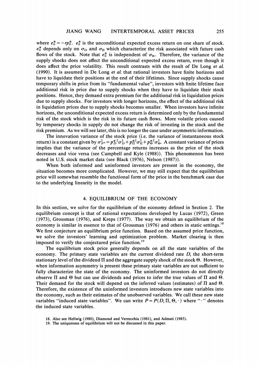
JIANG WANG INTERTEMPORAL ASSET PRICES 255 where e=-rpa.e is the unconditional expected excess return on one share of stock. e depends only on op and on which characterize the risk associated with future cash flows of the stock.Note that e is independent of oe.Therefore,the variance of the supply shocks does not affect the unconditional expected excess return,even though it does affect the price volatility.This result contrasts with the result of De Long et al. (1990).It is assumed in De Long et al.that rational investors have finite horizons and have to liquidate their positions at the end of their lifetimes.Since supply shocks cause temporary shifts in price from its "fundamental value",investors with finite lifetime face additional risk in price due to supply shocks when they have to liquidate their stock positions.Hence,they demand extra premium for the additional risk in liquidation prices due to supply shocks.For investors with longer horizons,the effect of the additional risk in liquidation prices due to supply shocks becomes smaller.When investors have infinite horizons,the unconditional expected excess return is determined only by the fundamental risk of the stock which is the risk in its future cash flows.More volatile prices caused by temporary shocks in supply do not change the risk of investing in the stock and the risk premium.As we will see later,this is no longer the case under asymmetric information. The innovation variance of the stock price (i.e.the variance of instantaneous stock return)is a constant given byop=p+pon+p.A constant variance of prices implies that the variance of the percentage returns increases as the price of the stock decreases and vice versa (see Campbell and Kyle (1988)).This phenomenon has been noted in U.S.stock market data(see Black(1976),Nelson(1987)). When both informed and uninformed investors are present in the economy,the situation becomes more complicated.However,we may still expect that the equilibrium price will somewhat resemble the functional form of the price in the benchmark case due to the underlying linearity in the model. 4.EQUILIBRIUM OF THE ECONOMY In this section,we solve for the equilibrium of the economy defined in Section 2.The equilibrium concept is that of rational expectations developed by Lucas (1972),Green (1973),Grossman (1976),and Kreps (1977).The way we obtain an equilibrium of the economy is similar in essence to that of Grossman(1976)and others in static settings. We first conjecture an equilibrium price function.Based on the assumed price function, we solve the investors'learning and optimization problem.Market clearing is then imposed to verify the conjectured price function.19 The equilibrium stock price generally depends on all the state variables of the economy.The primary state variables are the current dividend rate D,the short-term stationary level of the dividend II and the aggregate supply shock of the stock However, when information asymmetry is present these primary state variables are not sufficient to fully characterize the state of the economy.The uninformed investors do not directly observe II and but can use dividends and prices to infer the true values of II and Their demand for the stock will depend on the inferred values (estimates)of II and Therefore,the existence of the uninformed investors introduces new state variables into the economy,such as their estimates of the unobserved variables.We call these new state variables "induced state variables".We can write P=P(D,II,,.where"."denotes the induced state variables. 18.Also see Hellwig (1980),Diamond and Verrecchia(1981),and Admati(1985) 19.The uniqueness of equilibrium will not be discussed in this paper
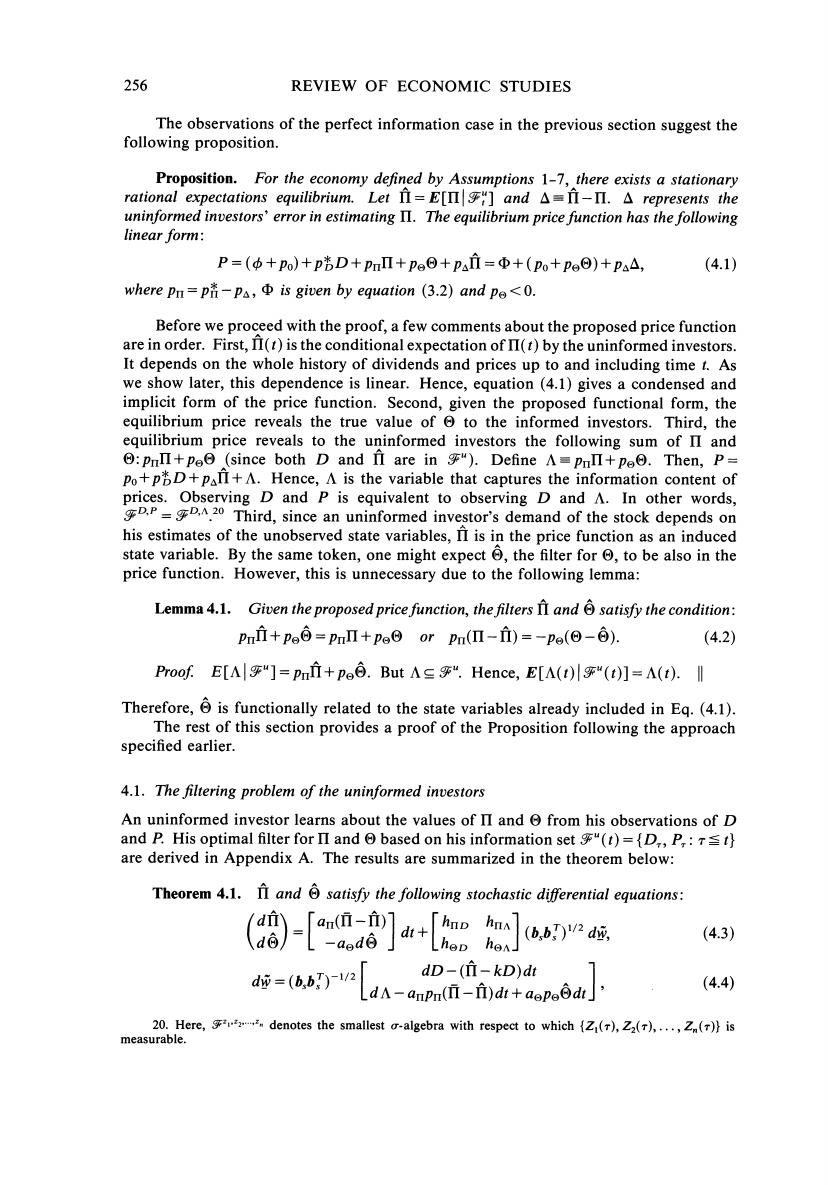
256 REVIEW OF ECONOMIC STUDIES The observations of the perfect information case in the previous section suggest the following proposition. Proposition.For the economy defined by Assumptions 1-7,there exists a stationary rational expectations equilibrium.Let II=E[II]and A=II-II.A represents the uninformed investors'error in estimating II.The equilibrium price function has the following linear form: P=(中+po)+pD+pmΠ+peΘ+Pai=Φ+(po+po⊙)+pa△, (4.1) where pn=p-pa,is given by equation (3.2)and pe<0. Before we proceed with the proof,a few comments about the proposed price function are in order.First,II(t)is the conditional expectation of II(t)by the uninformed investors. It depends on the whole history of dividends and prices up to and including time t.As we show later,this dependence is linear.Hence,equation(4.1)gives a condensed and implicit form of the price function.Second,given the proposed functional form,the equilibrium price reveals the true value of to the informed investors.Third,the equilibrium price reveals to the uninformed investors the following sum of II and o:pmΠ+peo(since both D and II are in“).Define A=pulΠ+peoo.Then,P- Po+pD+PanI+A.Hence,A is the variable that captures the information content of prices.Observing D and P is equivalent to observing D and A.In other words, 20 Third,since an uninformed investor's demand of the stock depends on his estimates of the unobserved state variables,II is in the price function as an induced state variable.By the same token,one might expect the filter for to be also in the price function.However,this is unnecessary due to the following lemma: Lemma 4.1.Given the proposed price function,the filters andsatisfy the condition: pmi+pg⊙=pmΠ+pg0orpm(Π-i)=-pa(⊙-⊙) (4.2) Proof.E[Ar“]=pmi+po日.But As“.Hence,E[A(t)lr“(t)]=A(t).I Therefore,is functionally related to the state variables already included in Eq.(4.1). The rest of this section provides a proof of the Proposition following the approach specified earlier. 4.1.The filtering problem of the uninformed investors An uninformed investor learns about the values of II and from his observations of D and P.His optimal filter for II and based on his information set"(t)={D,,P,:st} are derived in Appendix A.The results are summarized in the theorem below: Theorem 4.1.II and 6 satisfy the following stochastic differential equations: 8-[a8]+[e]” (4.3) dD-(f-kD)dt LdA-anpn(II-f)dt+aoPe0dt] (4.4) 20.Here,denotes the smallest a-algebra with respect to which (()Z(),...,Zn())is measurable
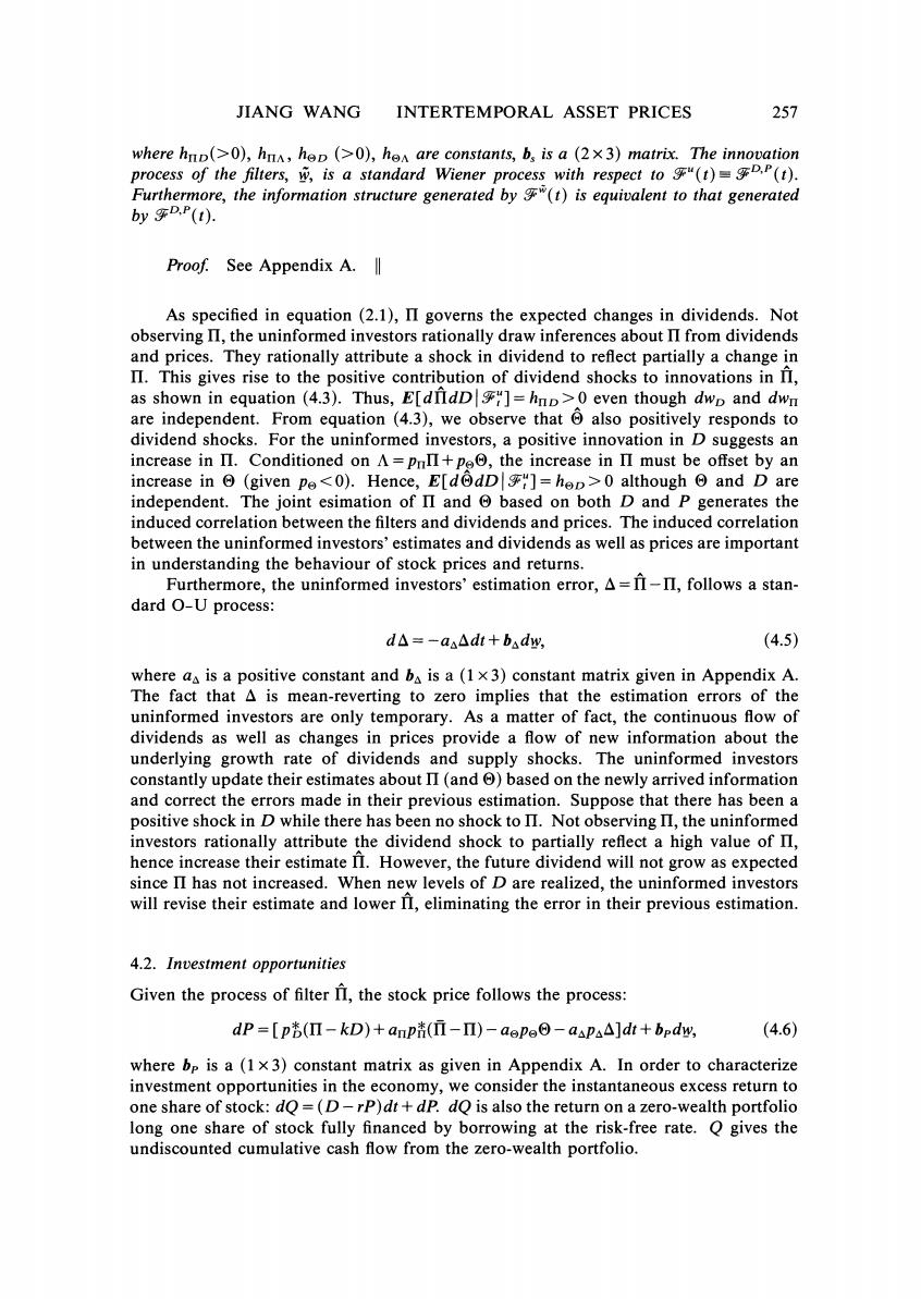
JIANG WANG INTERTEMPORAL ASSET PRICES 257 where hnp(>0),hun,hep (>0),hen are constants,b,is a (2x3)matrix.The innovation process of the filters,w,is a standard Wiener process with respect to g"(t)DP(t). Furthermore,the information structure generated by(t)is equivalent to that generated by D.P(t). Proof.See Appendix A. As specified in equation(2.1),II governs the expected changes in dividends.Not observing II,the uninformed investors rationally draw inferences about II from dividends and prices.They rationally attribute a shock in dividend to reflect partially a change in II.This gives rise to the positive contribution of dividend shocks to innovations in II, as shown in equation (4.3).Thus,E[dnIdD]=hnp>0 even though dwp and dwn are independent.From equation (4.3),we observe that also positively responds to dividend shocks.For the uninformed investors,a positive innovation in D suggests an increase in II.Conditioned on A=PnII+pe,the increase in II must be offset by an increase in (given pe<0).Hence,E[dodD]=hep>0 although and D are independent.The joint esimation of II and based on both D and P generates the induced correlation between the filters and dividends and prices.The induced correlation between the uninformed investors'estimates and dividends as well as prices are important in understanding the behaviour of stock prices and returns. Furthermore,the uninformed investors'estimation error,A=II-II,follows a stan- dard O-U process: d△=-aa△dt+badw, (4.5) where as is a positive constant and ba is a(1 x 3)constant matrix given in Appendix A. The fact that A is mean-reverting to zero implies that the estimation errors of the uninformed investors are only temporary.As a matter of fact,the continuous flow of dividends as well as changes in prices provide a flow of new information about the underlying growth rate of dividends and supply shocks.The uninformed investors constantly update their estimates about II(and )based on the newly arrived information and correct the errors made in their previous estimation.Suppose that there has been a positive shock in D while there has been no shock to II.Not observing II,the uninformed investors rationally attribute the dividend shock to partially reflect a high value of II, hence increase their estimate II.However,the future dividend will not grow as expected since II has not increased.When new levels of D are realized,the uninformed investors will revise their estimate and lower II,eliminating the error in their previous estimation. 4.2.Investment opportunities Given the process of filter II,the stock price follows the process: dP=[p(Π-kD)+anpt(i-I)-aePe⊙-aapa△]dt+bpdw, (4.6) where bp is a(1 x 3)constant matrix as given in Appendix A.In order to characterize investment opportunities in the economy,we consider the instantaneous excess return to one share of stock:dQ=(D-rP)dt+dp.dQ is also the return on a zero-wealth portfolio long one share of stock fully financed by borrowing at the risk-free rate.Q gives the undiscounted cumulative cash flow from the zero-wealth portfolio
258 REVIEW OF ECONOMIC STUDIES Theorem 4.2.Given the price process in equation (4.6),Q satisfies the stochastic differential equation: dQ=(D-rP)dt+dp=[eo+ee+eA]dt+bpdw, (4.7) where eo=-rpo,ee=-(r+ae)pe and ea=-(r+as)pa. To the informed investors,E[dQ]/dt eo+ee+eA.The expected excess return on the stock only depends on and A.The level of aggregate stock supply affects the excess return on the stock because it determines the total risk exposure of the economy. The short-run stationary level of dividend II does not affect the excess return per se,but A,the uninformed investors'error in estimating II,does.When A>0,the uninformed investors are over-estimating the future dividend growth,which drives up the price today. Future corrections are expected when information is revealed through new realizations of dividends.Hence,a price drop is expected by the informed investors.Therefore,the return expected by informed investors is negatively related to A(since ea<0).To the uninformed investors,E[dQ]/dt =eo+ee.Their expected excess return on the stock depends only on 0,their estimate of the supply shock. Theorem 4.2 simplifies the investors'optimization problems which we turn to next. Since the expected return on the stock is governed by and A,both following univariate processes,they fully determine the investment opportunities of the economy.21 4.3.The informed investors'optimization problem Let w be an informed investor's wealth,X'his holding of the stock and c'his consumption.His optimization problem is Maxi-ds s.t.dwi=(rwi-c')dt+x'dQ. (4.8) LetJ'(Wi;⊙,△;t)be the value function where⊙and△are the two state variables that govern the investment opportunities.J'satisfies the following Bellman equation:22 0=Maxc.x{-eor-c'+E[dJ(w;o,△;t)l(t)]/d s.t.dw=(rw-c')dt+X'dQ, Iim,oE[J'(W,⊙,△;t+r)川乎'(t)]=0. (4.9) The solution is provided in the following theorem:23 Theorem 4.3.Equation (4.9)has a solution of the form: J'(W;0,△;t)=-et-rw-v(o.a). (4.10) Here,V'(⊙,△)is a quadratic function:V'(Θ,△)=ΨTv业,where业r=(1,L,△).The optimal demand of the stock is a linear function of⊙and△: X'=fΨ (4.11) Here,v'and f=(fo,fe,fh)are respectively (3x3)and (1x3)constant matrices. Proof.See Appendix B. 21.The risk-free rate is assumed to be constant. 22.We assume that J is twice differentiable in its variables. 23.This problem is similar to the one solved by Merton(1971).The difference is that here we have two state variables governing the excess returns on the stock while Merton considers the single-variable case