
Implementing Statistical Criteria to Select Return Forecasting Models model selection criteria were employed:the adjusted R2,Akaike's infor- mation criterion [AIC;Akaike (1974)],Schwarz's criterion [a Bayesian information criterion,BIC;Schwarz (1978)],the Fisher information crite- rion [FIC;Wei(1992)],the posterior information criterion [PIC;Phillips and Ploberger (1996)],Rissanen's predictive least squares criterion [PLS; Rissanen (1986a)],2 and our adjustment to correct well-known biases of the latter,PLS-MDC. Appendix A provides formal definitions of each of these criteria.The adjusted R2,AIC,and BIC were chosen on the basis of their popularity; FIC,PIC,PLS,and PLS-MDC were chosen because of their robustness in the face of unit-root nonstationarities. PLS-MDC is new and hence needs to be motivated further.It is based on a technique to estimate the dimension of the state vector in Markov models,referred to as Markov dimension criterion (MDC).MDC chooses the dimension of the state vector by investigating the out-of-sample mean square prediction error of rolling regressions that are run on the basis of various subsets of past information. In conjunction with PLS,MDC provides a correction for small-sample biases.PLS chooses models on the basis of the out-of-sample mean square prediction error of one rolling regression that uses all past observations. Rissanen (1986a)suggested this selection criterion,but observed that it is biased in small samples in favor of picking the model with the least possible variables [see also the evidence in Wei (1992)].The underfitting is due to the noise introduced by the error in the predictions of early observations in the sample.These predictions are unreliable because they are based on very few prior observations (remember that model estimates in PLS are computed only from prior observations).The fewer parameters to be esti- mated,however,the lower the prediction noise of those early observations. Because of the lower noise level,PLS tends to prefer models with fewer parameters,that is,with less explanatory variables. In PLS-MDC,we consider the performance of the same models where parameter estimates are not only based on all previous observations,but on different subsamples as well,where we drop observations that reach a certain age.In other words,while PLS is based on expanding-window estimation, PLS-MDC also considers estimates based on windows of fixed size.PLS- MDC effectively penalizes models where excluded variables are still heavily correlated with future prediction errors,indicating that the prediction vector was chosen to be too small.Since a formal discussion of PLS-MDC distracts from the main points of this article,it is delegated to an appendix.The interested reader can consult Appendix B. 2 PLS is based on Rissanen's earlier idea of minimum descriptive length [Rissanen (1986b)]:see also Kavalieris (1989). 409

The Review of Financial Studies /v 12n 2 1999 As mentioned before,the purpose of statistical model selection criteria is to avoid overfitting.The model specification that fits the data best(minimum in-sample forecast error)is not necessarily chosen.In contrast,the retained model will have maximum external validity.In our context of return pre- diction,this means that the preferred model will have best out-of-sample forecasting performance. We decided to verify the external validity of formal model selection whenever k*>1.All models with index(k)larger than one contain at least one nontrivial forecasting variable.When one of them is chosen,the model selection criterion clearly supports predictability.To assess the external validity of such a conclusion,we ran a test on a sample that postdated the sample on which we based the model choice.To avoid confusion we will refer to the original sample on which model choice was based as the training sample.The sample that was used to check for external validity will be called the testing sample.The latter has size n,and its elements are indexed tT+1,...,T+n. External validation is investigated by projecting the market's excess re- turn,r,onto our forecast,-1.-1 is obtained from model k*,as follows: -1=1x二 (2) where is the OLSestimate of,based on the pairs ()observed over r =1....t-1.We estimate the slope coefficient in =Q+Bz1-I+, (3) from the observations indexed tT+1,...,T+n.We use the OLS estimate of B to compute a standard t-ratio,and refer to the standard normal distribution to determine p-levels.External validity is confirmed if p-levels are low,say,below 0.05. Notice that we did not adjust the t-ratio for error in the estimation of the parameters of the prediction model.Asymptotically,such an adjustment is not necessary,because we force the precision of the parameter estimates to increase as we advance through the testing sample.See also West(1996). Unfortunately,small-sample corrections are not available and would be complicated by the unit-root nature of some of the predictors. 3.The Data We investigated the predictability of the 1-month local-currency excess stock return for 14 countries.3 Our forecasts of the market's excess return is based on (a subset of)the following predictors:a January dummy;the Results can be expected to be different if excess stock returns are converted to a common currency.in which case retums from speculation in the foreign exchange market determine the outcome as well.See, for example,Ferson and Harvey (1993). 410

Implementing Statistical Criteria to Select Return Forecasting Models monthly excess stock return,lagged once and twice;a monthly bond excess return,lagged once and twice;*the yield-to-maturity on a representative Treasury bond;the stock market's price level;the yield-to-maturity on a 3- month Treasury bill (also used to compute excess stock and bond returns); the stock market's dividend yield;and the stock market's price-earnings ratio.None of these predictors use information that would not have been available at the moment that future excess stock returns were predicted. Appendix C provides a list of the data sources. Table I displays descriptive statistics of the monthly excess stock returns and the predictors.The lengths of the samples(T+n)run from a minimum of 122 observations (Norway)to a maximum of 471 observations(United States).Returns are expressed in percent per month;yields in percent per year.Table I also lists the beginning of the estimation sample for each country (t =1).Our choice was based on data availability,and hence was purely incidental. To get an idea of the amount of predictability that obtains in this dataset using in-sample statistical analysis,Table 2 lists the results from a regression of monthly excess stock returns (now not expressed in percentage terms) onto (i)an intercept,(ii)a January dummy,(iii)the stock dividend yield, (iv)the short-term interest rate,and (v)the long-term bond yield.Solnik (1993)also reports these estimates,for a similar dataset,but a shorter time period.The results of regressions like the ones reported in Table 2 match those of Solnik when run over his subperiod only (1/71-8/90).There is one exception though:our bond yield has more predictive power than his. A closer look at Table 2 reveals the patterns that Solnik discussed at length:predictability is not uniform across stock markets [R2s are between 2%(Germany)and 9.8%(U.K.)];predictors vary.The well-known nega- tive correlation between excess stock returns and contemporaneous interest rates is significant(at the 1%level)only for Belgium,France,and the United States. An unfortunate choice of subperiod,however,may give one the wrong impression of the amount of predictability.We tried one possible subsample and generated impressive evidence of predictability.Table 2 reports the results from estimation of the same regression over the subperiod 1/71- 8/80(10 years shorter than Solnik's sampling period).They are listed under Period II.The R2s run from a low of 4.4%(Canada)to a high of 36.4% (Belgium)or higher!Overall,the significance of the coefficients in the regression is overwhelming. 4This bond return is actually computed from the yield on a representative Treasury bond and an estimate of the duration.Hence it cannot strictly be considered to be a bond (excess)return.Nevertheless,its computation does not require future information.Therefore it is a proper predictor. 5 Some high R2s may be the result of lack of observations.The highest R2,40%(Spain).is based on a sampling period that runs from 1/78 to 8/80 only.Belgium's high R2.however,is based on a full sample. 411
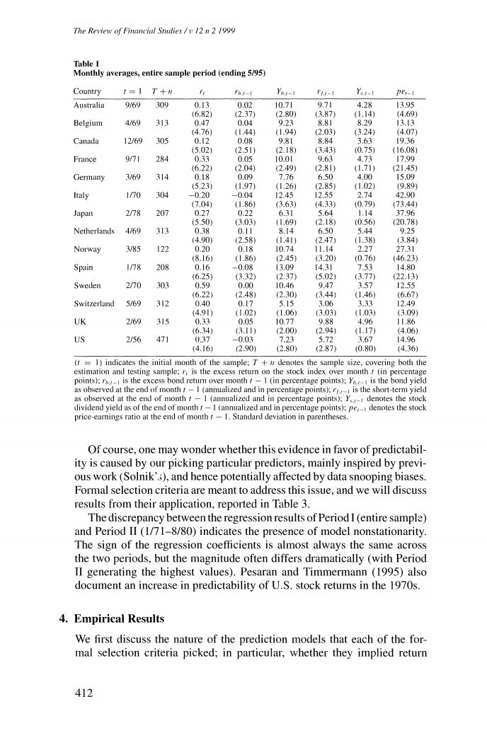
The Review of Financial Studies /v 12 n 2 1999 Table I Monthly averages,entire sample period (ending 5/95) Country 1=1 T+ I6J-1 Yh.t-1 -1 YsI-I per-1 Australia 9/69 309 0.13 0.02 10.71 9.71 4.28 13.95 (6.82) (2.37 (2.80) (3.87) (1.14) (4.69) Belgium 4/69 313 0.47 0.04 9.23 8.81 8.29 1313 (4.76) (1.44) (1.94) 2.03) (3.24) (4.07) Canada 12/69 305 0.I2 0.08 9.81 8.84 3.63 19.36 (5.02) (2.51) (2.18) (3.43) 0.75) (16.08) France 971 284 0.33 0.05 10.01 9.63 4.73 17.99 (6.22) (2.04) (2.49) (2.81) (1.71) (21.45) Germany 3/69 314 0.18 0.09 7.76 6.50 4.00 15.09 (5.23) (1.97) (1.26) (2.85) (1.02) (9.89) Italy 170 304 -0.20 -0.04 12.45 12.55 2.74 42.90 (7.04 (1.86) (3.63) (4.33) (0.79) (73.44) Japan 2/78 207 0.27 0.22 6.31 5.64 1.14 37.96 (5.50) (3.03 (1.69) (2.18) (0.56 (20.78) Netherlands 4/69 313 0.38 0.11 8.14 6.50 5.44 9.25 14.90 (2.58) (1.41) (2.47) (1.38) (3.84 Norway 3/85 122 0.20 0.18 10.74 11.14 2.27 27.31 (8.16) (1.86) (2.45 (3.20) (0.76) (46.23) Spain 1/78 208 0.16 -0.08 13.09 14.31 7.53 14.80 (6.25 (3.32) (2.37) (5.02) (3.77 (22.13) Sweden 270 303 0.59 0.00 10.46 9.47 3.57 12.55 (6.22) (2.48) (2.30) (3.44) (1.46) (6.67) Switzerland 5/69 312 0.40 0.17 5.15 3.06 3.33 12.49 (4.91) 41.02) (1.06) (3.03) (1.03) (3.09) UK 2/69 315 0.33 0.05 10.77 988 4.96 11.86 (6.34) 3.11) (2.00 (2.94) (1.17) (4.06) US 2/56 471 0.37 -0.03 7.23 5.72 3.67 14.96 (4.16) (2.90) (2.80) (2.87) (0.80) (4.36) (t=1)indicates the initial month of the sample:7+#denotes the sample size,covering both the estimation and testing sample:is the excess return on the stock index over month t(in percentage points):is the excess bond return over month t-I (in percentage points);Y is the bond yield as observed at the end of month /-I (annualized and in percentage points);r,is the short-term yield as observed at the end of month r-I (annualized and in percentage points);Y denotes the stock dividend yield as of the end of month f-I (annualized and in percentage points):pe,_denotes the stock price-earnings ratio at the end of month t-1.Standard deviation in parentheses Of course,one may wonder whether this evidence in favor of predictabil- ity is caused by our picking particular predictors,mainly inspired by previ- ous work (Solnik'3),and hence potentially affected by data snooping biases. Formal selection criteria are meant to address this issue,and we will discuss results from their application,reported in Table 3. The discrepancy between the regression results of Period I(entire sample) and Period II (1/71-8/80)indicates the presence of model nonstationarity. The sign of the regression coefficients is almost always the same across the two periods,but the magnitude often differs dramatically (with Period II generating the highest values).Pesaran and Timmermann (1995)also document an increase in predictability of U.S.stock returns in the 1970s. 4.Empirical Results We first discuss the nature of the prediction models that each of the for- mal selection criteria picked;in particular,whether they implied return 412