E.Normalization We return now to the statistical interpretation of the wave function,which says that (,)2is the probability density for finding the particle at point r,at time t.It follows that the integral of(,)must be 1 (the particle's got to be somewhere) (2) If(t)is a solution of Schrodinger equation,so too are Av(,t)and e(,).Here A is any complex constant,a is a phase factor of the wave function.What we must do,then,is pick this undetermined multiplicative factor so as to ensure that Equation(2)is satisfied. This process is called normalizing the wave function.For some solutions to the Schrodinger equation,the integral is infinite;in that case no multiplicative factor is going to make it 1. The same goes for the trivial solution(,t)=0.Such non-normalizable solutions cannot represent particles,and must be rejected.Physically realizable states correspond to the square-integrable"solutions to Schrodinger's equation. Erample:Problem 1.4 on page 14 of Griffiths At timet=0,a particle is represented by the wave function A话,if0≤x≤a (x,0)= A,ifa≤E≤b 0, otherwise where A,a and b are constants. (a)Normalize(that is,find A,in terms of a and b). (b)Sketch(,0)as a function of z. (c)Where is the particle most likely to be found,att=0? (d)What is the probability of finding the particle to the left of a?Check your result in the limiting cases b=a and b=2a. (e)What is the expectation value of r? Solution: 16
E. Normalization We return now to the statistical interpretation of the wave function, which says that |ψ(x, t)| 2 is the probability density for finding the particle at point x, at time t. It follows that the integral of |ψ(x, t)| 2 must be 1 (the particle’s got to be somewhere) Z +∞ −∞ |ψ(x, t)| 2 dx = 1 (2) If ψ(x, t) is a solution of Schr¨odinger equation, so too are Aψ(x, t) and e iαψ(x, t). Here A is any complex constant, α is a phase factor of the wave function. What we must do, then, is pick this undetermined multiplicative factor so as to ensure that Equation (2) is satisfied. This process is called normalizing the wave function. For some solutions to the Schr¨odinger equation, the integral is infinite; in that case no multiplicative factor is going to make it 1. The same goes for the trivial solution ψ(x, t) = 0. Such non-normalizable solutions cannot represent particles, and must be rejected. Physically realizable states correspond to the ”square-integrable” solutions to Schr¨odinger’s equation. Example: Problem 1.4 on page 14 of Griffiths. At time t = 0, a particle is represented by the wave function ψ(x, 0) = A x a , A b−x b−a , 0, if 0 ≤ x ≤ a if a ≤ x ≤ b otherwise where A, a and b are constants. (a) Normalize ψ (that is, find A, in terms of a and b). (b) Sketch ψ(x, 0) as a function of x. (c) Where is the particle most likely to be found, at t = 0? (d) What is the probability of finding the particle to the left of a? Check your result in the limiting cases b = a and b = 2a. (e) What is the expectation value of x? Solution: 16
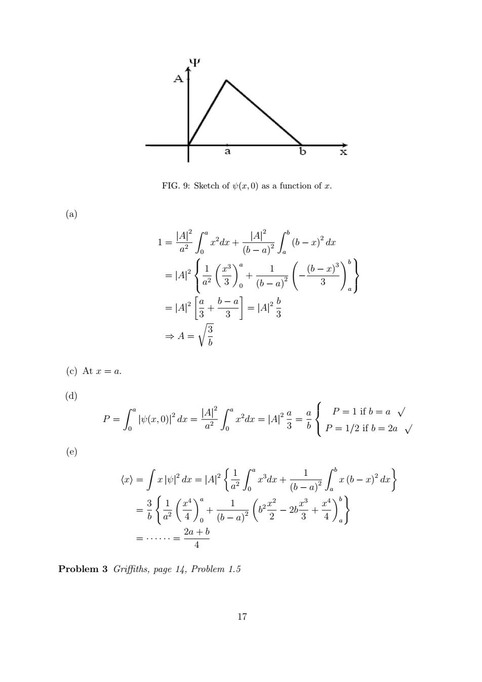
FIG.9:Sketch of (,0)as a function of 创 1-g+- -4G+g-ar号 →A=V停 (c)At r=a (d) -eaa-g-r号- -∫rt=4r{侣k+o可o- =()+(号-号+ =…=2a+b 4 Problem 3 Griffiths,page 14,Problem 1.5 17
FIG. 9: Sketch of ψ(x, 0) as a function of x. (a) 1 = |A| 2 a 2 Z a 0 x 2 dx + |A| 2 (b − a) 2 Z b a (b − x) 2 dx = |A| 2 1 a 2 µ x 3 3 ¶a 0 + 1 (b − a) 2 Ã − (b − x) 3 3 !b a = |A| 2 · a 3 + b − a 3 ¸ = |A| 2 b 3 ⇒ A = r 3 b (c) At x = a. (d) P = Z a 0 |ψ(x, 0)| 2 dx = |A| 2 a 2 Z a 0 x 2 dx = |A| 2 a 3 = a b P = 1 if b = a √ P = 1/2 if b = 2a √ (e) hxi = Z x |ψ| 2 dx = |A| 2 ½ 1 a 2 Z a 0 x 3 dx + 1 (b − a) 2 Z b a x (b − x) 2 dx¾ = 3 b ( 1 a 2 µ x 4 4 ¶a 0 + 1 (b − a) 2 µ b 2 x 2 2 − 2b x 3 3 + x 4 4 ¶b a ) = · · · · · · = 2a + b 4 Problem 3 Griffiths, page 14, Problem 1.5 17
III.MOMENTUM AND UNCERTAINTY RELATION In classical mechanics,we learn that position and momentum are canonical variables to each other.In 1D case,this can be seen from the Fourier transformation and its reverse 1 [too (x,)= pp,t)e严d 1 pp,)=2x元J- (a,t)e-严dr A.Expectation value of dynamical quantities For a particle in state (r),the expectation/mean/average value of r is =广te,rP在=eG0we,0血 What exactly does this mean?It emphatically does not mean that if you measure the position of one particle over and over again,dr is the average of the results you'll get.On the contrary,the first measurement(whose outcome is indeterminate)will collapse the wave function to a spike at the value actually obtained,and the subsequent measurements (if they're performed quickly)will simply repeat that same result.Rather,()is the average of measurements performed on particles all in the state which means that either you must find some way of returning the particle to its original state after each measurement,or else you prepare a whole ensemble of particles,each in the same state and measure the positions of all of them:(is the average of these results. In short,the erpectation value is the average of repeated measurements on an ensemble of identically prepared systems,not the average of repeated measurements on one and the same system. Similarly one can get the expectation value of the potential energy V() we》=vae,Pz=e,voee在 But for the momentum p,this is not true 创≠(z,),r 18
III. MOMENTUM AND UNCERTAINTY RELATION In classical mechanics, we learn that position and momentum are canonical variables to each other. In 1D case, this can be seen from the Fourier transformation and its reverse ψ(x, t) = 1 √ 2π~ Z +∞ −∞ ϕ(p, t)e i ~ pxdp ϕ(p, t) = 1 √ 2π~ Z +∞ −∞ ψ(x, t)e − i ~ pxdx A. Expectation value of dynamical quantities For a particle in state ψ(x), the expectation/mean/average value of x is hxi = Z +∞ −∞ x |ψ(x, t)| 2 dx = Z +∞ −∞ ψ ∗ (x, t) xψ (x, t) dx What exactly does this mean? It emphatically does not mean that if you measure the position of one particle over and over again, R x |ψ| 2 dx is the average of the results you’ll get. On the contrary, the first measurement (whose outcome is indeterminate) will collapse the wave function to a spike at the value actually obtained, and the subsequent measurements (if they’re performed quickly) will simply repeat that same result. Rather, hxi is the average of measurements performed on particles all in the state ψ, which means that either you must find some way of returning the particle to its original state after each measurement, or else you prepare a whole ensemble of particles, each in the same state ψ, and measure the positions of all of them: hxi is the average of these results. In short, the expectation value is the average of repeated measurements on an ensemble of identically prepared systems, not the average of repeated measurements on one and the same system. Similarly one can get the expectation value of the potential energy V (x) hV (x)i = Z +∞ −∞ V (x)|ψ(x, t)| 2 dx = Z +∞ −∞ ψ ∗ (x, t) V (x)ψ (x, t) dx But for the momentum p, this is not true hpi 6= Z +∞ −∞ ψ ∗ (x, t) ψ (x, t) pdx 18

Instead,by means of the Fourier transformation of the wave function,(p,t),we have (p)(p.)e(p.pdp-"p.pe(p.)dp -中(高款eer)en dpire (epe(r.) d 1 Collecting the underlined terms into(,t),we have 创-w(-)c刊 Definition:For ID case,the momentum operator is defined as and +oo )=、p,0心,) It is straightforward to generalize the Fourier transformation result to 3D case (r,t)= 1 (p.t)eiordp 1 p.)=2史 v(r,t)e-pd The corresponding momentum operators are defined as p=-访V with the components =-h品=-协=-品 For simplicity we introduce 0,约)三0= 19
Instead, by means of the Fourier transformation of the wave function, ϕ(p, t), we have hpi = Z +∞ −∞ ϕ ∗ (p, t)ϕ(p, t)pdp = Z +∞ −∞ ϕ ∗ (p, t)pϕ(p, t)dp = Z +∞ −∞ dp µZ +∞ −∞ dx 1 √ 2π~ ψ ∗ (x, t) e i ~ px¶ pϕ(p, t) = 1 √ 2π~ Z Z +∞ −∞ dpdxψ∗ (x, t) e i ~ pxpϕ(p, t) = Z Z +∞ −∞ dxdpψ ∗ (x, t) µ −i~ d dx¶ 1 √ 2π~ e i ~ pxϕ(p, t) Collecting the underlined terms into ψ (x, t), we have hpi = Z +∞ −∞ dxψ∗ (x, t) µ −i~ d dx¶ ψ (x, t) Definition: For 1D case, the momentum operator is defined as pˆ = −i~ d dx and hpi = Z +∞ −∞ ψ ∗ (x, t) ˆpψ (x, t) dx 6= Z +∞ −∞ ψ ∗ (x, t) ψ (x, t) ˆpdx It is straightforward to generalize the Fourier transformation result to 3D case ψ (r, t) = 1 (2π~) 3/2 ZZZ +∞ −∞ ϕ(p, t)e i ~ p·r d 3p ϕ(p, t) = 1 (2π~) 3/2 ZZZ +∞ −∞ ψ(r, t)e − i ~ p·r d 3 r The corresponding momentum operators are defined as pb = −i~∇ with the components pˆx = −i~ ∂ ∂x, pˆy = −i~ ∂ ∂y , pˆz = −i~ ∂ ∂z For simplicity we introduce (ψ, ψ) ≡ Z dτψ∗ψ = Z dτ |ψ| 2 19

where dr means dr for 1D,drdydz for 3D,and drdydz...drndyNdzN for N particles. The normalization takes a very simple form (,)=1 The mean value of a dynamical quantity A is If the wave function is not normalized we should compute it as (o,Ao】 Problem 4 Consider a particle in one dimensional system.Both the wave function(,t) and its Fourier transformation(p,t)can represent the state of the particle. (r,t)is the wave function (or state function, probability amplitude)in position representation (p,t)represents the same state in momentum representation,just like a vector can be erpressed in different coordinate systems If we use(p,t)to represent the state,what are the operatorsr and p?p is just p itself,but what about x? B.Examples of uncertainty relation Let us examine again the example of Gaussian wave packets -()” It is localized in momentum about p=hko.We can check the normalization 20
where dτ means dx for 1D, dxdydz for 3D, and dx1dy1dz1 · · · dxN dyN dzN for N particles. The normalization takes a very simple form (ψ, ψ) = 1 The mean value of a dynamical quantity A is hAi = ZZZ +∞ −∞ ψ ∗ (r, t) Aψˆ (r, t) d 3 r = ³ ψ, Aψˆ ´ If the wave function is not normalized we should compute it as hAi = ³ ψ, Aψˆ ´ (ψ, ψ) Problem 4 Consider a particle in one dimensional system. Both the wave function ψ(x, t) and its Fourier transformation ϕ(p, t) can represent the state of the particle. ψ(x, t) is the wave function (or state function, probability amplitude) in position representation ϕ(p, t) represents the same state in momentum representation, just like a vector can be expressed in different coordinate systems If we use ϕ(p, t) to represent the state, what are the operators x and p? p is just p itself, but what about x? B. Examples of uncertainty relation Let us examine again the example of Gaussian wave packets ϕ(k) = µ 2α π ¶1/4 e −α(k−k0) 2 . It is localized in momentum about p = ~k0. We can check the normalization Z +∞ −∞ |ϕ(k)| 2 dk = r 2α π Z +∞ −∞ e −2α(k−k0) 2 dk = r 2α π r π 2α = 1 20